Introduction
Chapter 1 covered a lot of ground. It had to. Before building anything, we needed to survey what already exists - over fifty tools across five categories, decades of published neuroscience linking brain activation to content performance, the specific gap that no one has bridged, and the three bets the project exists to test. That was necessary homework: you cannot lay out a formal framework without first establishing what it stands on and what it stands apart from. All of that is now behind us. This is where we actually start building.
This chapter gives the ambition from Chapter 1 its mathematical bones. It defines the formal vocabulary, the logical structures, and the analytical tools that every subsequent chapter uses. By the end, the reader will be able to name the six empirical facts the framework rests on, navigate the four domains it operates in, trace how information flows between those domains, understand what Khozai computes and why, and use thirteen formal operations for discovering, testing, and validating claims.
What the reader will learn. Six premises about the brain’s hardware. Four mathematical spaces describing the domains of operation. Five mappings describing how information flows. The vector architecture that defines what Khozai computes. Thirteen reasoning tools for discovery, characterization, and validation. Explicit scope boundaries marking where the framework stops and why.
Why. Every claim in this book traces back to the structures defined in this chapter. If a claim cannot be grounded here, it is either unjustified or requires expanding this foundation. The framework is designed to be self-correcting: its own tools validate its evidence, catch its contradictions, and extend its scope when gaps appear.
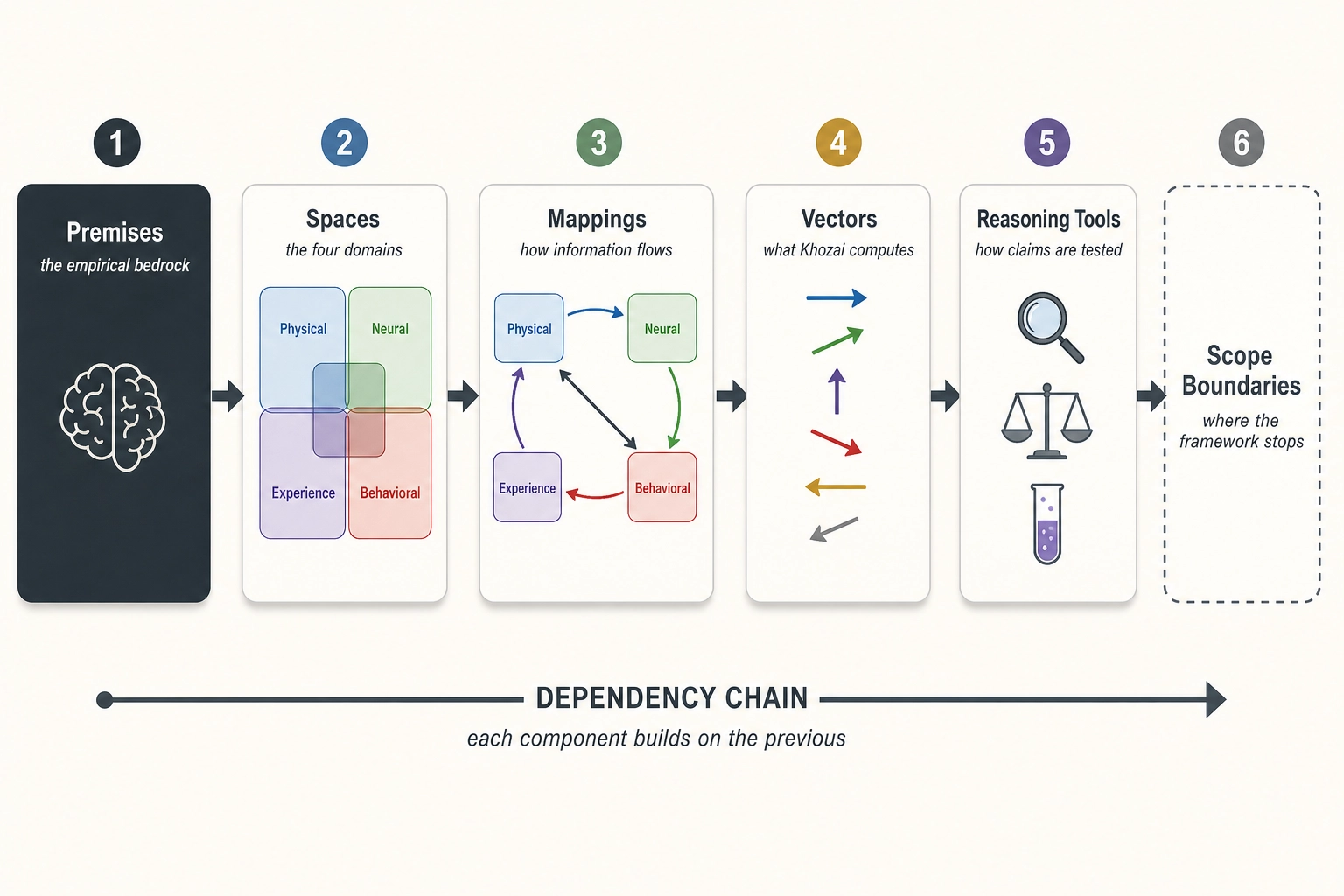
How the chapter is organized. The chapter follows a dependency chain. Section 1 lays the empirical bedrock (premises). Section 2 defines the domains those premises create (spaces). Section 3 describes how information flows between domains (mappings). Section 4 introduces what Khozai computes within those domains (vectors). Section 5 provides the analytical operations for working within the framework (reasoning tools). Section 6 draws the boundary around what the framework can and cannot claim (scope and derived principles).
1. Premises
A premise in this framework is a factual statement about the physical world that is empirically established, experimentally replicable, and not derived from other statements in the framework. Premises are the bedrock. If a premise is wrong, everything derived from it must be re-examined. If a needed claim cannot be traced to a premise, either the claim is unjustified or a new premise is needed. This section defines the six premises and their evidence. It does not discuss how the framework formalizes them into mathematical objects (that is Section 2) or what Khozai computes from them (that is Section 4).
The six premises are not independent of each other. Premise 1 establishes that experience exists. Premises 2, 3, and 4 establish that the hardware producing it is finite and catalogued. Premise 5 connects structure to experience: specific hardware produces specific aspects. Premise 6 connects structure to behavior: specific hardware produces specific outputs. Together, they license the decomposition of experience into measurable dimensions and the decomposition of behavior into measurable outcomes.
1.1. Premise 1 - Experience Exists
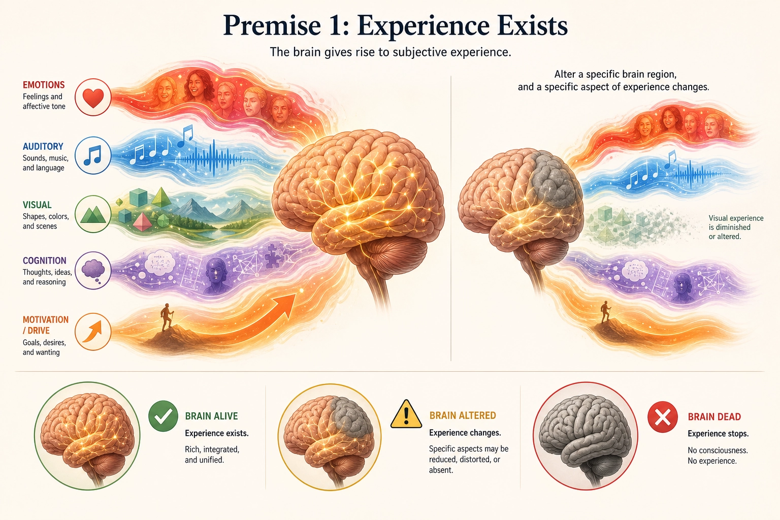
Statement: A living human brain produces subjective experience.
Grounding: Every living human reports subjective experience. Removing the brain eliminates it: clinical brain death criteria define death as the irreversible cessation of all brain function, after which no capacity for experience remains (Wijdicks et al., 2010 [20]). Altering the brain alters it: general anesthetics acting on the brain reliably abolish and restore consciousness in a dose-dependent manner (Alkire, Hudetz & Tononi 2008 [15]). These observations are universal and replicable. The research program built on this premise - identifying the specific neural mechanisms that produce specific conscious experiences - was formally launched by Crick and Koch (1990) [19] and has generated thousands of studies since.
The word “produces” in the statement is a theoretical commitment, not a neutral observation. The evidence establishes dependence: experience depends on the brain, covaries with brain states, and disappears when the brain ceases to function. Whether this dependence is best described as production, as identity (experience IS brain activity), or as something else is a philosophical question the framework does not settle. Eliminative materialists would say there is no “experience” to produce - only neural processes we mislabel. Panpsychists would say experience is fundamental, not produced. The framework requires only the dependence: that brain states and experiential states systematically covary, and that altering one alters the other. That dependence is empirically established regardless of which philosophical interpretation is correct.
What this says: Brain alive - experience exists. Brain dead - experience stops. Brain altered - experience changes.
What this does NOT say: It does not say what experience IS (the hard problem). It does not say how the brain produces it. It does not say anything about non-human experience. It establishes existence, not mechanism.
1.2. Premise 2 - Receptors Are Finite and Complete
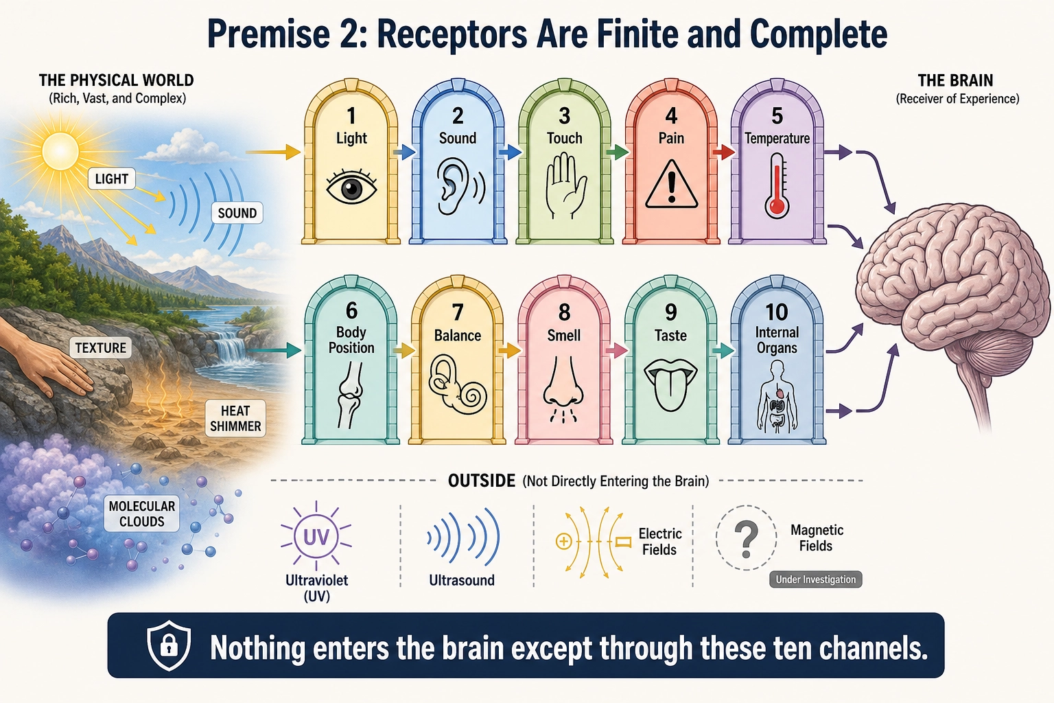
Statement: The brain has a finite and complete set of receptor systems that transduce physical energy into neural signals. As categorized here, there are ten major receptor systems in humans.
A note on categorization. The number ten reflects one defensible way to draw the boundaries. Some of these categories are cleaner than others. Photoreceptors and cochlear hair cells transduce well-defined physical dimensions (electromagnetic radiation, pressure waves). Nociceptors are less clean: “tissue damage” is not a physical dimension in the same sense - nociceptors respond to excessive mechanical, thermal, and chemical stimulation across modalities. Thermoreceptors and nociceptors overlap (some nociceptors fire on extreme temperature). Visceral afferents are a grab-bag category spanning several transduction mechanisms. A different but equally defensible categorization might count 8 or 12. What matters for the premise is not the exact number but that the set is finite and the major systems are all identified. The framework’s logic holds whether the count is 8, 10, or 12.
The ten receptor systems:
| # | Receptor System | In Simple Terms | Physical Dimension Transduced | Receptor Types |
|---|---|---|---|---|
| 1 | Photoreceptors | Light sensors in the eye | Electromagnetic radiation (380-700nm) | Rods, L/M/S cones |
| 2 | Cochlear hair cells | Sound sensors in the inner ear | Air pressure waves (20-20,000 Hz) | Inner and outer hair cells |
| 3 | Mechanoreceptors | Touch and pressure sensors in the skin | Mechanical deformation of tissue | Meissner, Pacinian, Merkel, Ruffini |
| 4 | Nociceptors | Pain sensors throughout the body | Tissue damage signals | Aδ mechanical, Aδ thermal, C polymodal |
| 5 | Thermoreceptors | Temperature sensors in the skin | Thermal energy | Warm receptors, cold receptors |
| 6 | Proprioceptors | Body-position sensors in muscles and joints | Muscle/tendon stretch and joint angle | Muscle spindles, Golgi tendon organs, joint receptors |
| 7 | Vestibular organs | Balance sensors in the inner ear | Angular and linear acceleration | 3 semicircular canals, 2 otolith organs |
| 8 | Olfactory receptors | Smell sensors in the nose | Airborne molecules | ~400 receptor types |
| 9 | Gustatory receptors | Taste sensors on the tongue | Dissolved molecules | Type II (sweet/bitter/umami), Type III (sour), ion channels (salt) |
| 10 | Visceral afferents | Internal organ sensors | Internal organ state | Mechanoreceptors, chemoreceptors, osmoreceptors in organs |
Grounding: Receptor systems are physical biological hardware identified through anatomy, histology, and molecular biology [1]. The list is complete in the same way the list of human organs is complete: the major systems are all identified, though mechanisms within them continue to be refined. The Piezo channel discovery (2010) identified the molecular mechanism of mechanoreception, not a new sensory modality [2]. One active area of investigation is human magnetoreception: the neuroscientist Connie Wang et al. (2019) [34] found that controlled rotations of an Earth-strength magnetic field produced repeatable alpha-wave desynchronization in human EEG (electroencephalography, a method of recording electrical activity from the scalp), suggesting a transduction mechanism for geomagnetic fields. If confirmed and replicated, this would add an 11th modality. The finding has not yet been independently replicated, and no receptor has been identified, so the framework treats ten as the current count - but the premise is designed to accommodate additions. A new modality would extend the list, not break the framework.
What this says: The brain’s input from the physical world comes through these channels. There is no perception without transduction. The list represents the current complete inventory - ten established modalities, with magnetoreception under investigation.
What this does NOT say: It does not say each receptor system produces a distinct experiential state (that requires testing). It does not say anything about how the brain processes these signals after transduction.
1.3. Premise 3 - Cortical Organization Is Hierarchical and Multi-Resolution
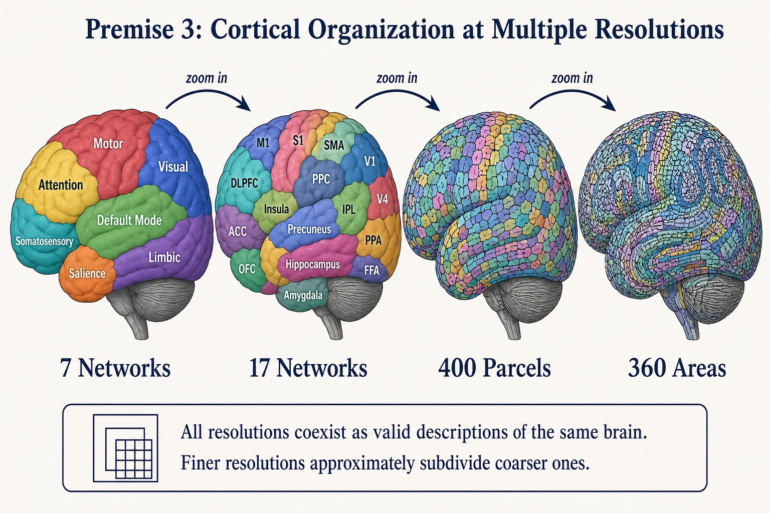
Statement: The brain’s cortex is composed of a finite set of anatomically distinct regions (~52 areas originally identified by the neuroanatomist Korbinian Brodmann in 1909 [3], refined to 180 areas per hemisphere - 360 total - by the neuroanatomist Matthew Glasser and colleagues in 2016 [4]). These regions organize into functional networks whose neural activity is more correlated within networks than between them. This organization is observable at multiple resolutions.
Multi-resolution structure:
| Resolution | Number of Networks | Source | What It Captures |
|---|---|---|---|
| Coarse | 7 networks | The neuroscientist B.T. Thomas Yeo and colleagues (2011) [5] | Broadest functional divisions |
| Fine | 17 networks | Yeo et al. (2011) [5] | Finer functional subdivisions |
| Parcel | ~400 parcels | The neuroscientist Alexander Schaefer and colleagues (2018) [6] | Individual functional regions |
| Area | ~360 areas | Glasser et al. (2016) [4] | Multi-modal cortical areas |
Grounding: Yeo and colleagues (2011) [5] applied clustering analysis to resting-state fMRI (functional magnetic resonance imaging, which measures brain activity by detecting blood-flow changes) data from 1,000 subjects. The resulting network solutions are stable across individuals and populations. The method groups regions by correlation: regions with more correlated firing patterns form one network, regions with less correlated patterns form separate networks. The 7-network and 17-network solutions have been replicated across independent datasets (Schaefer et al. 2018 [6] used a separate sample of 1,489 subjects), across imaging modalities (task-based fMRI, diffusion tractography, and MEG produce convergent network boundaries), and across populations (the Human Connectome Project confirmed the same network architecture across 1,200 subjects with higher-resolution imaging).
On hierarchy and nesting. The statement says “multi-resolution”: that multiple valid descriptions exist at different granularities. It is tempting to read this as clean hierarchical nesting, where finer resolutions subdivide coarser ones without contradiction. The reality is messier. The Yeo networks (functional connectivity), Schaefer parcels (functional connectivity at finer grain), and Glasser areas (multi-modal anatomical) use different methods and criteria. Schaefer parcels do not always nest cleanly within Yeo networks. A parcel may straddle two coarser networks, or a network boundary may shift depending on the method. The multi-resolution property is real - the brain’s organization can be described at multiple valid granularities - but “finer subdivides coarser” is an approximation, not a strict mathematical property. The framework uses it as a useful modeling assumption, not as a proven fact about cortical geometry.
On “decorrelation.” Between-network correlations are real and significant, especially during task performance. The clustering method minimizes between-network correlation relative to within-network correlation - it does not eliminate it. Networks interact extensively. The premise claims that networks are identifiable as distinct organizational units, not that they are independent systems.
What this says: Cortical networks are real, observable, finite, and organized at multiple resolutions. The number identified depends on the resolution of analysis, and multiple resolutions coexist as valid descriptions.
What this does NOT say: It does not claim one resolution is “correct.” It does not claim resolutions nest perfectly. It does not say each network produces a distinct experiential state (that requires testing). It does not describe subcortical structures (that is Premise 4).
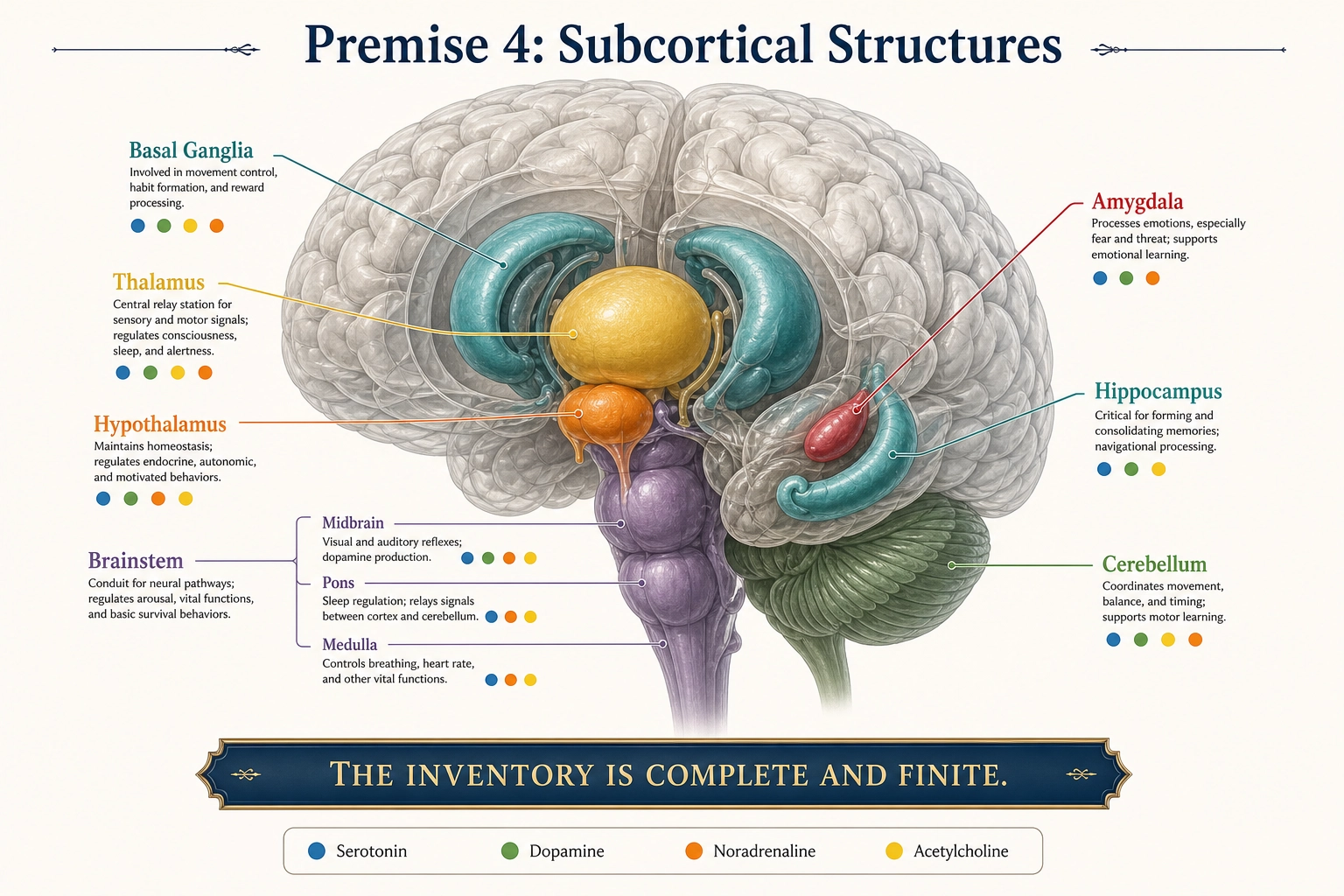
1.4. Premise 4 - Subcortical Structures Are Finite and Complete
Statement: The brain contains a finite and complete set of subcortical structures (the structures beneath the cortical surface), each anatomically identifiable and neurochemically characterized.
Full inventory:
- Diencephalon: Thalamus (LGN, MGN, pulvinar, mediodorsal, anterior, ventral lateral, ventral posterior, intralaminar, reticular nucleus); Hypothalamus (lateral, ventromedial, suprachiasmatic, preoptic, paraventricular, arcuate, supraoptic, dorsomedial); Epithalamus (habenula, pineal gland); Subthalamus (subthalamic nucleus)
- Basal ganglia: Caudate nucleus, putamen, globus pallidus (internal and external), nucleus accumbens (ventral striatum), ventral pallidum
- Limbic subcortical: Amygdala (basolateral, central, medial nuclei), hippocampal formation (CA1-CA4, dentate gyrus, subiculum, entorhinal cortex), bed nucleus of stria terminalis, septal nuclei
- Basal forebrain: Nucleus basalis of Meynert (cholinergic), medial septal nucleus (cholinergic), diagonal band of Broca
- Brainstem - Midbrain: Ventral tegmental area (dopaminergic), substantia nigra pars compacta (dopaminergic) and pars reticulata (GABAergic), superior colliculus, inferior colliculus, periaqueductal gray, red nucleus, pedunculopontine nucleus
- Brainstem - Pons: Locus coeruleus (noradrenergic), raphe nuclei - dorsal and median (serotonergic), parabrachial nucleus, pontine nuclei
- Brainstem - Medulla: Raphe nuclei - caudal group (serotonergic), nucleus tractus solitarius, rostral ventrolateral medulla, area postrema, reticular formation (ascending reticular activating system spans midbrain through medulla), inferior olivary nucleus
- Cerebellum: Cerebellar cortex (molecular, Purkinje, granular layers), deep cerebellar nuclei (dentate, interposed, fastigial)
- Other: Claustrum, pituitary gland (anterior and posterior)
Grounding: Subcortical structures are anatomical - identifiable through dissection, histology, and imaging in every human brain. The definitive stereotaxic atlas (a coordinate-based map of brain structures) of the human brain (Mai, Majtanik & Paxinos 2016 [21]) maps every subcortical region through cytoarchitectonic and myeloarchitectonic analysis (specialized histological methods for identifying brain regions by their cell structure and nerve fiber patterns). The Allen Human Brain Atlas (Hawrylycz et al. 2012 [22]) independently confirmed this inventory through systematic gene-expression mapping across approximately 500 samples per hemisphere, organized into a closed hierarchical ontology covering all cortical and subcortical structures. The inventory is complete in the same way the receptor list (Premise 2) is complete.
What this says: The subcortical brain is made of these structures and only these structures.
What this does NOT say: It does not group them into functional systems (that is a derived step). It does not say which ones produce experiential states versus which modulate or relay (that requires testing with the Classification Test, Tool 5, defined in Section 5).
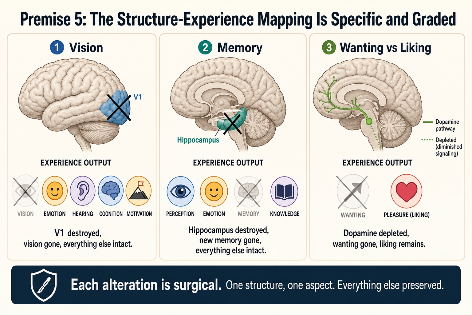
1.5. Premise 5 - The Structure-Experience Mapping Is Specific and Graded
Statement: Altering specific neural structures alters specific aspects of experience while leaving other aspects intact. Specific aspects can be fully eliminated by destruction of their underlying structures without eliminating other aspects. The relationship is graded: partial alteration produces partial change.
Grounding:
Lesion studies: V1 destruction (primary visual cortex, the first cortical area to process visual signals) produces cortical blindness with all other experience intact. the neurologist Gordon Holmes (1918) [23] demonstrated this through systematic analysis of focal occipital lesions, showing that the size and location of V1 damage maps precisely to the size and location of the resulting blind region in the visual field - a direct demonstration of specific and graded structure-experience correspondence. Hippocampal destruction (patient HM) produces amnesia with perception, emotion, and cognition intact [7].
Pharmacological dissociation: In rodents, dopamine depletion eliminates wanting (effortful pursuit of reward) while preserving liking (hedonic reactions to reward), a double dissociation demonstrated by the neuroscientists Kent Berridge and Terry Robinson (1998) [8] and replicated extensively in animal models. The human picture is less clean: there is no validated human analog to the orofacial “liking” measure used in rodents, self-report conflates wanting with expected pleasure, and human neuroimaging shows overlapping rather than fully separable circuits (the psychologist Eva Pool and colleagues 2016 [30]). Berridge himself has noted that humans cannot reliably distinguish wanting from liking introspectively [31]. The framework uses this dissociation as evidence that experience has separable components with distinct neural substrates - a principle well-established in rodents and supported by indirect human evidence (addiction studies, dopamine manipulation), even though the sharp mechanistic separation demonstrated in animal models has not been replicated with equivalent rigor in humans.
Graded stimulation: Stronger motor cortex stimulation produces stronger muscle contraction (Penfield & Boldrey 1937 [9]). Larger V1 lesions produce larger visual field loss (Holmes 1918 [23]). In rodents, higher dopamine antagonist doses produce greater reduction in wanting (Berridge & Robinson 1998 [8]) - though as noted above, the human translation of this specific grading is less well-established.
What this says: Experience has separable components that map to specific neural structures. The mapping is specific (not random) and graded (not binary). This is the premise that makes Experience Space decomposable and makes the entire project of finding independent experiential dimensions possible.
What this does NOT say: It does not explain HOW neural structures produce experience (the hard problem). It does not specify how many components there are or what they are (that requires systematic testing). It does not say the mapping is 1:1 - one structure can contribute to multiple aspects, and one aspect can depend on multiple structures.
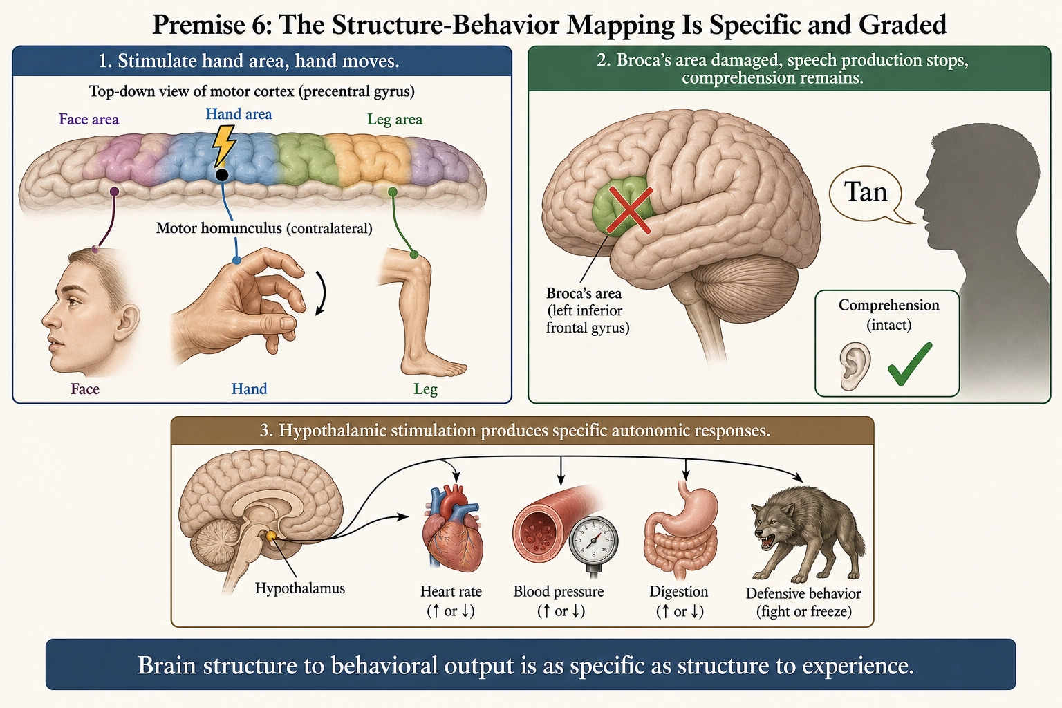
1.6. Premise 6 - The Structure-Behavior Mapping Is Specific and Graded
Statement: The brain produces behavioral output through specific neural structures. Specific structural activation produces specific motor, physiological, and communicative responses. The mapping is observable, specific, and graded.
Grounding:
The neurosurgeon Wilder Penfield and the neurologist Edwin Boldrey (1937) [9]: Electrical stimulation of specific motor cortex regions produces specific muscle contractions, mapped across hundreds of patients. Replicated and extended across thousands of subsequent studies using direct cortical stimulation, TMS (transcranial magnetic stimulation - a non-invasive method of stimulating the brain through the skull), and fMRI.
Lesion evidence: Motor cortex damage produces paralysis of specific body parts. the physician Paul Broca (1861) [24] documented patient Leborgne, who could comprehend speech but produce only a single syllable, with post-mortem examination localizing the damage to the left inferior frontal gyrus. This became the founding case for brain-behavior localization. However, modern re-examination of Leborgne’s preserved brain using high-resolution MRI (Dronkers et al. 2007 [32]) revealed that the lesion extended well beyond the cortical surface into deep white matter and the superior longitudinal fasciculus - far more extensive subcortically than Broca’s gross examination could detect. This complicates the clean “one region, one function” narrative: damage to Broca’s area alone does not always eliminate speech production, and comprehension deficits sometimes accompany it. What the evidence does establish - and what the premise requires - is that the mapping from brain structure to behavioral output is specific and graded, even if the specificity operates at the level of distributed circuits rather than single cortical regions.
Autonomic: the physiologist Walter Hess (1949) [25] demonstrated through systematic electrical stimulation of discrete hypothalamic sites that specific locations produce specific, reproducible autonomic and behavioral responses - increased heart rate and blood pressure from one site, decreased heart rate and increased gut motility from another, coordinated feeding or defensive behaviors from others. Hess received the 1949 Nobel Prize in Physiology or Medicine for establishing that the hypothalamus contains a precise map of autonomic functions.
What this says: Behavioral output, like experience, maps to specific neural structures with specific and graded relationships. Behavioral output is objectively measurable by third-party observers.
What this does NOT say: It does not say whether experience is required for behavior (some behavior bypasses experience entirely). It does not describe the full space of possible behaviors (that is Space 4).
Six premises establish what the brain’s hardware IS: experience exists, the input channels are finite, the processing regions are finite and organized at multiple resolutions, the subcortical structures are finite, the structure-to-experience mapping is specific and graded, and the structure-to-behavior mapping is specific and graded. The next question: what mathematical objects describe the domains this hardware defines?
2. Spaces
The framework defines four mathematical spaces. Each space describes a domain in which the system operates. A “space” in this context is the complete set of all possible states of something - not a physical location, but a mathematical way of describing every configuration something could take. A space has dimensions (axes), points (specific configurations), and structure (how points relate to each other). All four spaces are multi-resolution: they can be described at multiple levels of granularity, and coarser descriptions are projections of finer ones. This section defines each space’s structure and properties. It does not describe how information flows between spaces (that is Section 3) or what Khozai computes within them (that is Section 4).
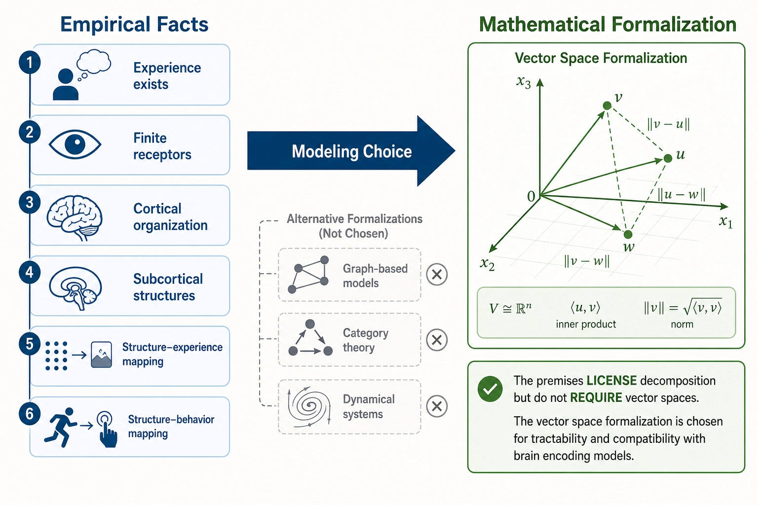
From facts to formalization. The premises establish empirical facts: finite hardware, decomposable experience, graded mappings. The spaces that follow are mathematical formalizations imposed on those facts - a modeling choice, not a logical entailment. The premises license decomposition: experience has separable aspects (Premise 5), the hardware producing them is finite (Premises 2-4). But representing those aspects as dimensions of a vector space - with axes, points, distances, and algebraic operations - is a decision to use a particular mathematical language. Other formalizations are possible: graph-based models, category theory, dynamical systems. The framework adopts the vector space formalization because it is well-understood, computationally tractable, and directly compatible with the brain encoding models and machine learning tools Khozai uses. The reader should understand that the mathematical structure below is not discovered in the premises - it is chosen to represent what the premises establish, and it inherits the assumptions that vector space formalization brings (continuity, linearity of combination, metric structure). Where those assumptions may not hold, this is noted in the relevant space definition.
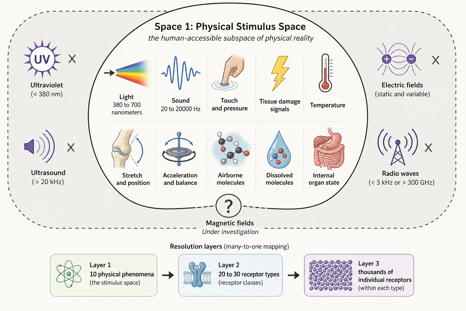
2.1. Space 1 - Physical Stimulus Space
Definition: The human-accessible subspace of physical reality. The set of all physical energy configurations that human receptor systems can transduce (convert from physical energy into neural signals).
Grounding: Premise 2 (receptors are finite and complete).
Dimensionality: Multi-resolution. All resolutions coexist as valid descriptions:
| Resolution | Axes | What Each Axis Represents |
|---|---|---|
| Physical phenomenon | ~10 | Each distinct physical dimension transduced by a receptor system (electromagnetic radiation, pressure waves, mechanical deformation, etc.) |
| Receptor type | ~20-30 | Each distinct receptor type within the ten systems (L-cone, M-cone, S-cone, rods, Meissner, Pacinian, etc.) |
| Individual receptor channel | Thousands | Each individual receptor unit (each hair cell at each cochlear position, each photoreceptor at each retinal position, etc.) |
Mathematical properties:
- Functions as a vector space: stimuli can be added and scaled, axes are physically independent (changing electromagnetic radiation does not necessitate changing pressure waves).
- Finite-dimensional at every resolution.
- Axes at the physical phenomenon level are physically incommensurable (they measure fundamentally different things that cannot be converted into each other): electromagnetic radiation and pressure waves have no common unit.
- Higher resolutions subdivide lower resolutions approximately: receptor types (L-cone, M-cone, S-cone) sit within the broader photoreceptor axis, but as noted in Premise 3, clean hierarchical nesting is an idealization.
Scope note: This space describes what physical energy CAN reach the organism. Dimensions of physical reality that no established human receptor can detect (ultraviolet radiation, ultrasound, electric fields) are outside this space. Magnetic fields are a borderline case: preliminary evidence for human magnetoreception exists (Premise 2, Wang et al. 2019 [34]) but is not yet independently replicated, so the current space definition excludes them.
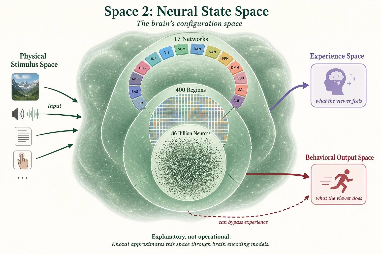
2.2. Space 2 - Neural State Space
Definition: The space of all possible configurations of the brain’s hardware at a given moment. A point in this space is a complete specification of activity across all neural structures.
Grounding: Premises 3 (cortical organization) and 4 (subcortical structures).
Dimensionality: Multi-resolution:
| Resolution | Axes | Source |
|---|---|---|
| Neuron level | ~86 billion | Every neuron’s firing rate |
| Region level | ~400 | Average activity per cortical/subcortical region |
| Network level | ~17 (cortical) + subcortical systems | Overall activation per functional network |
Role in framework: Explanatory, not operational. Neural State Space is what PRODUCES Experience Space (Premise 5) and what MEDIATES between Physical Stimulus Space and Behavioral Output Space. Khozai does not directly compute in this space - it approximates it through brain encoding models (AI systems trained on real fMRI data that predict which brain regions would activate in response to a given stimulus, without needing a scanner or subjects). These models and the vectors they produce are defined in section 4.
What it grounds: The Dissociation Test (Tool 1, section 5) works because different structures in this space can be independently altered (Premises 3, 4, 5). Experience Space is finite-dimensional because this space is finite (Premises 2, 3, 4). Experience Space is approximately hierarchical because neural processing in this space is organized at multiple resolutions (Premise 3) - though as noted in Premise 3, the nesting is an approximation rather than a strict mathematical property.
Operational properties note: The brain’s operational properties (inhibition, always-on processing, bidirectional connectivity, state-dependent processing, self-modification, no central control, multiple timescales) are properties of HOW this space operates, not of the space itself. They are detailed in Chapter 3 (The Brain’s Architecture) rather than in this space definition.
2.3. Space 3 - Experience Space
Definition: The space of all possible moments of subjective experience. A point in this space is the complete characterization of one instant of conscious experience.
Grounding: Premise 1 (experience exists) and Premise 5 (experience is decomposable: specific structural alterations eliminate specific aspects while leaving others intact).
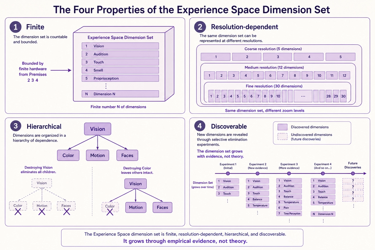
Dimensionality: A “dimension” in this space is one separable aspect of what a person can experience - something that can vary on its own, from fully present to fully absent, without requiring anything else to change along with it. Vision is a dimension: destroy the primary visual cortex and vision disappears while hearing, emotion, cognition, and motivation remain intact. Arousal is a dimension: damage the brainstem’s reticular activating system and the person slides toward coma while every other aspect of their experiential machinery remains structurally present. Each dimension is an aspect of experience that has been demonstrated through selective elimination (Premise 5) to be separable from other aspects. The dimension set is:
- Finite - bounded by the finite hardware that produces it (Premises 2, 3, 4).
- Resolution-dependent - finer resolution reveals more separable aspects. All resolutions coexist.
- Hierarchical - smaller dimensions live inside bigger ones, the way subfolders live inside folders. Color is a dimension inside vision. Destroy the vision hardware and you lose color, motion, faces, everything visual. Destroy only the color hardware and you lose color but keep the rest of vision intact. Broader dimensions contain their constituent narrower dimensions.
- Discoverable - each demonstrated selective elimination reveals a dimension. The dimension set grows with evidence, not with theory.
The number of dimensions depends on the resolution. Broader resolutions yield fewer dimensions (single digits), finer resolutions yield more (tens). The specific counts at each resolution, the evidence that earns each dimension its place, the alternative decompositions considered, and the hierarchy that organizes them is the work of Chapter 4.
Properties of each dimension:
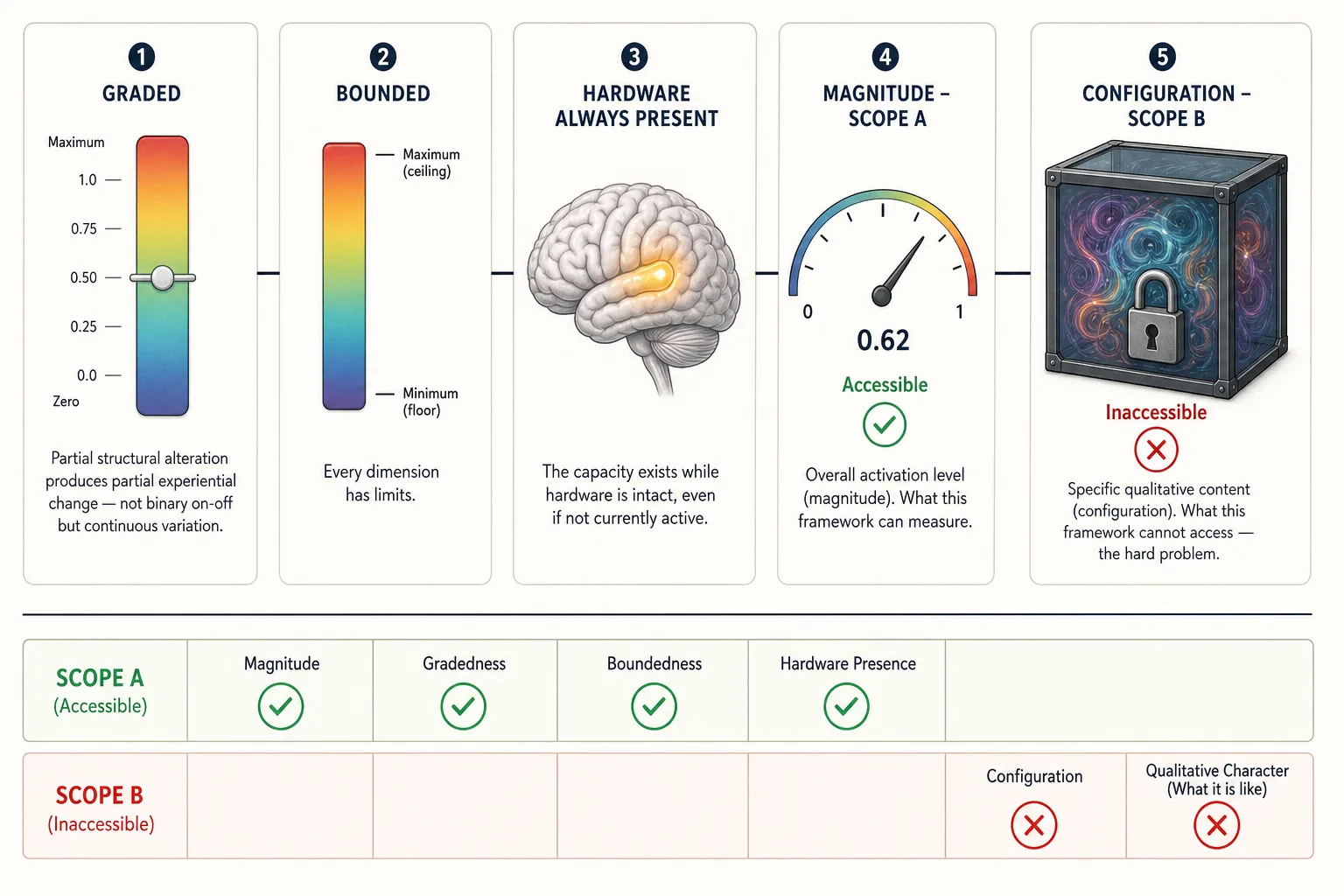
- Graded: partial structural alteration produces partial change (Premise 5). The framework models this as continuous variation, but this is a modeling assumption, not an established fact. Some aspects of experience show categorical properties - color perception is categorical despite continuous wavelength variation, pain has threshold effects, and consciousness itself may have discrete transitions (awake versus not). The continuous model is adopted because it is mathematically tractable and consistent with the graded evidence from Premise 5, but the reader should understand that “graded” (empirically demonstrated) and “continuous” (mathematically assumed) are not the same claim.
- Bounded: each dimension has a minimum (near-zero activation) and maximum.
- Hardware always present in an intact brain: while the underlying hardware is intact, the capacity for that dimension of experience exists. Whether the dimension is experientially “active” at any given moment is a separate question - the gustatory dimension’s hardware is intact while you read this, but you are unlikely to be having a taste experience right now. What the premise establishes is that the hardware is available and can be activated by appropriate stimulation. Destruction of the hardware eliminates the dimension entirely (Premise 5). The framework models dimensions as having a minimum activation level (near-zero), not as being always experientially engaged.
- Has magnitude: a scalar representing overall activation level at one instant. Magnitude is what the framework can approximate: how strongly a dimension is engaged.
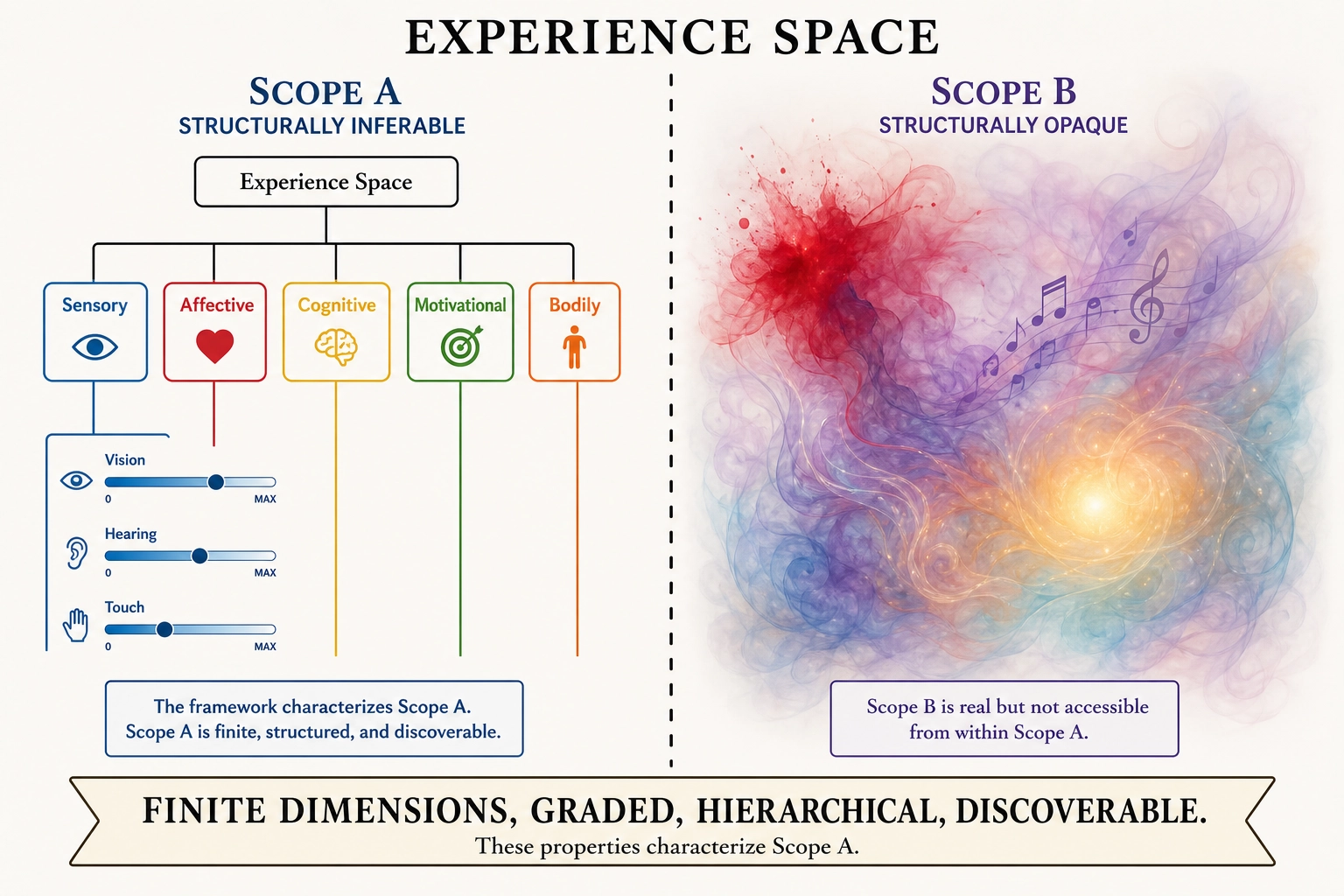
- Has configuration: the specific qualitative pattern within the dimension at one instant (what you are seeing, not just how much visual processing is happening). The hardware’s state, which specific neurons fire in which pattern, determines the configuration. That is Mapping 2 (Production, section 3), but the mechanism by which neural patterns become specific experiences is unknown. That is the hard problem of consciousness. Configuration is real but beyond the framework’s reach - we can know that the visual dimension is active, but not what the person is seeing. This boundary between what the framework can and cannot access is formalized below as Scope A (structurally inferable) versus Scope B (structurally opaque) of Experience Space.
| Property | What It Means | What the Framework Can Access |
|---|---|---|
| Graded | Partial alteration produces partial change | Yes - magnitude (Scope A) |
| Bounded | Minimum (near-zero) to maximum | Yes - range (Scope A) |
| Hardware always present | Capacity exists while hardware is intact | Yes - structural presence (Scope A) |
| Has magnitude | Scalar activation level at one instant | Yes - approximated through Vn and Ve |
| Has configuration | Specific qualitative pattern (what you see, not how much) | No - configuration is Scope B (the hard problem) |
Properties of the space:
- Approximately hierarchical: smaller dimensions generally live inside bigger ones (color inside vision, vision inside sensory). The hierarchy is determined by neural architecture, not philosophical categorization. As with cortical networks (Premise 3), the nesting is approximate - some dimensions may participate in multiple broader categories, and the boundaries between levels are not always clean.
- A point is instantaneous: describes one moment. Rate of change, history, and duration are properties of trajectories (curves through the space over time), not properties of points.
- Bounded: every dimension has a minimum and maximum.
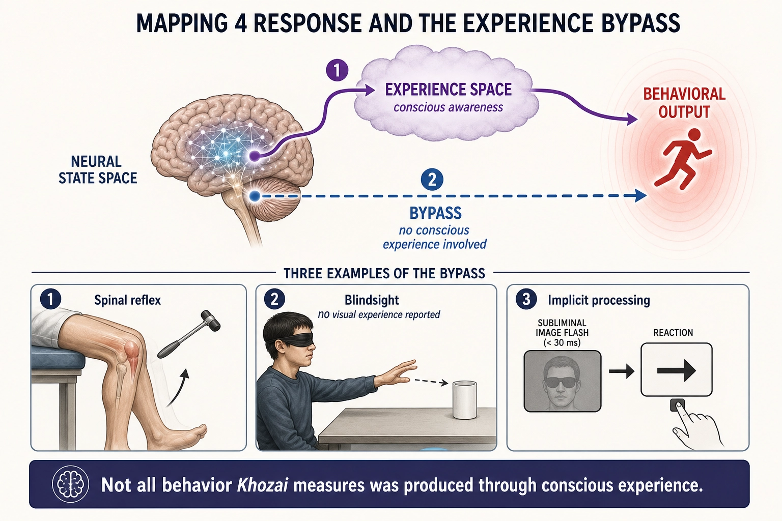
- Can be bypassed: some neural processing produces behavioral output without corresponding experience (reflexes, blindsight - where patients with destroyed visual cortex respond to visual stimuli despite reporting no visual experience - and implicit processing).
- Feeds back: a point in Experience Space influences Neural State Space (conscious awareness modulates subsequent neural processing).
Independence: Two dimensions are independent if and only if they are independently manipulable, demonstrated through the Dissociation Test (Tool 1, section 5). Independence means “one can change while the other is held constant,” shown through experimental evidence. Independence does NOT mean uncorrelated: independent dimensions frequently co-vary in natural conditions but CAN be separated under experimental manipulation.
The binding problem. Defining Experience Space as having separable dimensions raises a question that the framework must acknowledge: subjective experience is unified. You do not experience vision + hearing + emotion as separate channels running in parallel - you experience a single integrated scene. This is the binding problem: how do separately processed neural signals combine into a unified experience? The framework decomposes experience into dimensions because the neural evidence (Premise 5) demonstrates they can be independently eliminated. But that empirical separability does not explain how, in normal operation, they produce a unified whole. The framework’s decomposition describes what can be taken apart, not how the parts are put together. This is a second boundary alongside the hard problem: the framework characterizes the dimensions of experience but not the mechanism of their integration.
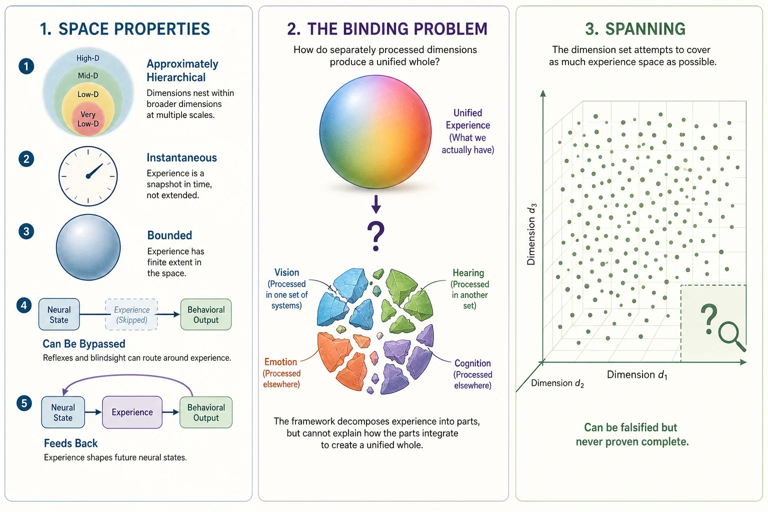
Spanning: The dimension set spans Experience Space if every possible moment of experience can be described as a point using only these dimensions with no residual. Spanning is testable through falsification: attempting to find experiences that cannot be described. It can never be proven complete, only survive repeated attempts to break it.
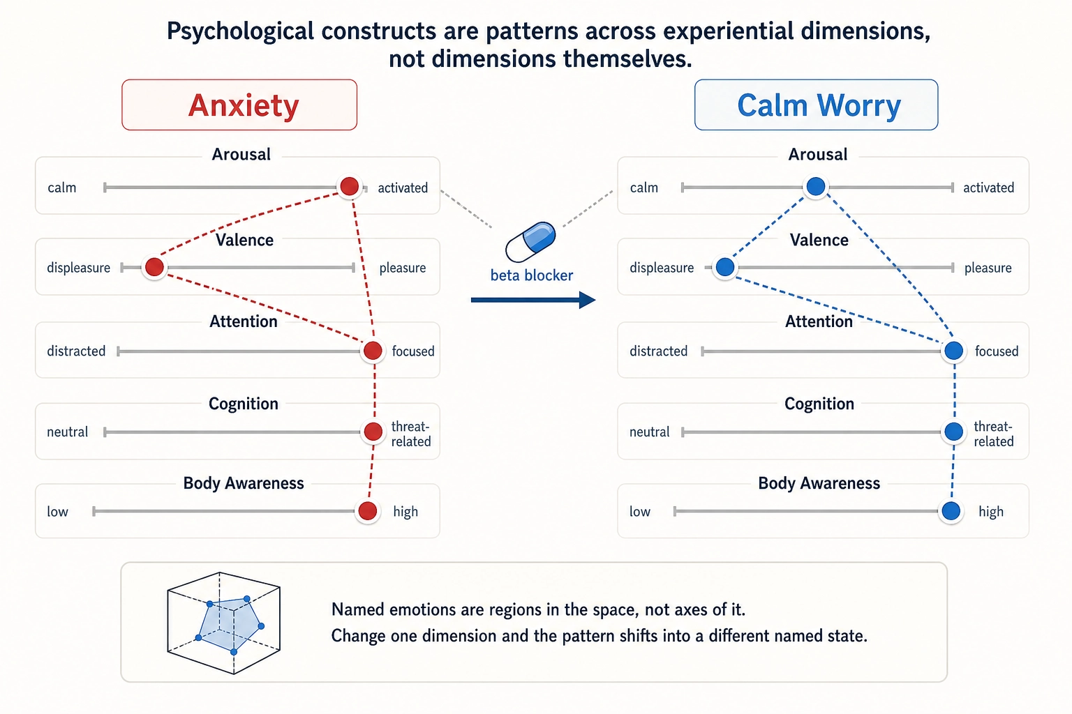
Relationship to psychology: Psychology has spent over a century naming states of human experience: anxiety, flow, nostalgia, awe, boredom, curiosity, grief, euphoria. These are real and useful names. But in this framework, they are not dimensions - they are patterns across dimensions. Anxiety, for example, is not a single axis you can turn up or down. It is a specific combination: high arousal, negative affect, heightened vigilance (attention), threat-related cognition, and elevated body-state awareness, all occurring together. Change any one of those components and the experience shifts into something else. Give someone a beta blocker (which lowers arousal) and the anxiety becomes something calmer - the worry may remain but the racing heart and physical tension dissolve, and the person no longer calls it anxiety. That is the test: if altering one dimension transforms the named state into a different named state, the original was a pattern across dimensions, not a dimension itself (this is formalized as Tool 6, the Pattern Verification Test, in section 5). Psychology has been naming patterns in Experience Space for over a century. This framework provides the coordinate system underlying those patterns - the dimensions that combine to produce them.
Two scopes of Experience Space:
- Scope A - Structurally Inferable: The dimensions, their independence, their hierarchy, their gradedness. Accessible through Structural Inference (Mapping 3, section 3) from Neural State Space architecture. This is what the framework characterizes.
- Scope B - Structurally Opaque: The qualitative character of experience (qualia - what red looks like, what longing feels like), the unity of consciousness, the raw subjectivity of being an experiencer, the emergent qualities of dimensional combinations, and any aspects lacking identified neural correlates. Real (we experience them) but not accessible through this framework’s methodology. Acknowledged, not characterized.
A note on Neural State Space versus Experience Space. These two spaces describe the same brain from two different angles, and the reader may notice the chapter keeps connecting them. The distinction is fundamental. Neural State Space is the objective, physical state of the brain: which neurons are firing, which regions are active, which chemicals are flowing. It is measurable by an outside observer with instruments like fMRI or EEG. It is hardware doing things. Experience Space is the subjective experience that hardware produces: what the person actually perceives, feels, thinks, wants. It is accessible only from inside - no instrument can measure what red looks like to you. Same brain, two descriptions. One is the machine running. The other is what it is like to be that machine. The framework needs both because Khozai measures the first (through brain encoding models that predict neural activity from a video file) but ultimately cares about the second (because what the viewer experiences is what drives their response).
2.4. Space 4 - Behavioral Output Space
Definition: The space of all possible outputs the brain can produce that affect the body or the external world. A point in this space is the complete specification of all outputs at a given moment.
Grounding: Premise 6 (the brain produces behavioral output through specific structures, specific and graded).
Dimensionality: Multi-resolution. Axes defined by effector systems (the muscles, glands, and organs that carry out the brain’s commands):
| Resolution | In Simple Terms | Axes | Examples |
|---|---|---|---|
| Effector level | Every individual muscle, nerve, and gland | Thousands | Each motor unit, each autonomic nerve terminal, each endocrine gland |
| Output system level | Four broad categories of output | Four major systems | Motor, autonomic, endocrine, immune |
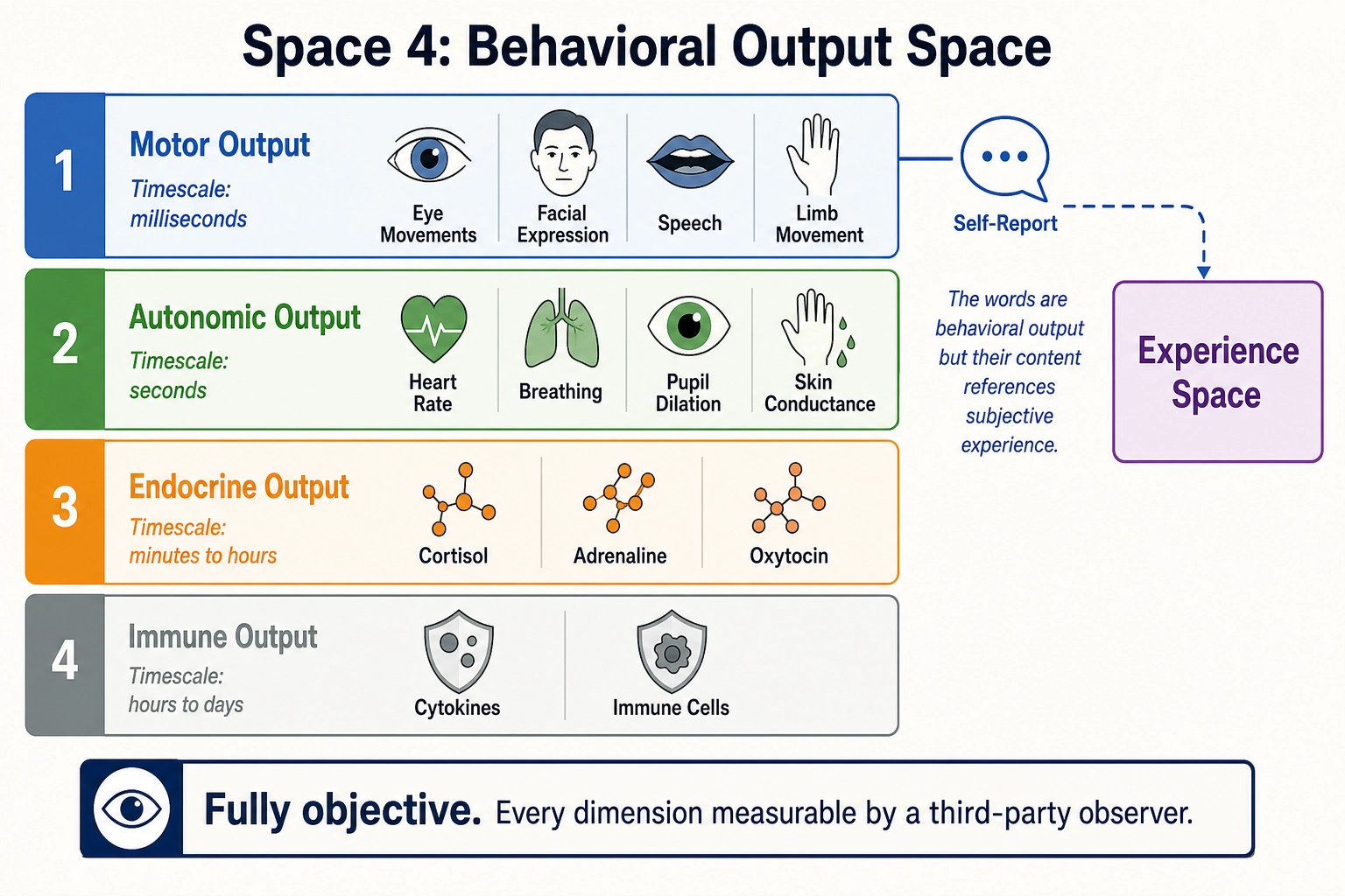
Four output systems:
- Motor output - skeletal muscle contractions. Sub-dimensions: eye movements, facial expression, vocal production, upper/lower limb, trunk, speech articulation. Timescale: milliseconds.
- Autonomic output - heart rate, breathing, pupil dilation, skin conductance, blood pressure, digestion, sexual arousal. Timescale: seconds.
- Endocrine output - cortisol, adrenaline, oxytocin, testosterone, insulin, melatonin. Timescale: minutes to hours.
- Immune output - cytokines, immune cell mobilization. Timescale: hours to days. Including immune output as “behavioral” is a stretch of the conventional meaning - the immune system is not typically classified as behavior. It is included here because the brain modulates immune function through autonomic and endocrine pathways, and immune state affects subsequent neural processing (sickness behavior, fatigue, mood changes). For Khozai’s purposes, immune output is the least operationally relevant category - it operates on timescales far longer than content viewing - but it is included for completeness of the brain’s output channels.
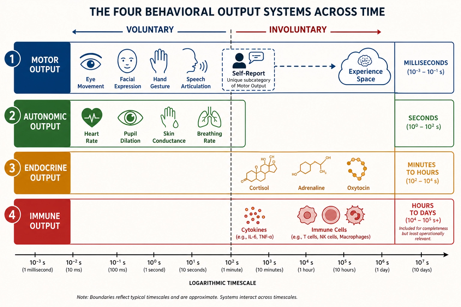
Self-report: the bridge to Experience Space. One category of behavioral output has a unique property: self-report. Physically, self-report is motor output (speech, typing, gesture), but its content REFERENCES Experience Space. When a viewer comments “this made me cry” or “I can’t stop watching,” they are producing behavioral output whose content describes their subjective experience. Self-report is the primary source of information about Scope B of Experience Space - what the viewer actually felt, not just which dimensions were structurally engaged. It is also how psychology has studied experience for over a century. Its limitations (filtered through language, biased by social desirability, limited by introspective access, selective, voluntary and sparse [10]) and its role in the framework are detailed in Chapter 6.
Properties:
- Finite-dimensional, continuous, graded.
- Multiple timescales across output systems.
- Partially voluntary (motor, self-report), partially involuntary (autonomic, endocrine, immune).
- Objectively measurable: unlike Experience Space, every dimension can be measured by a third-party observer.
- The only space whose motor output acts on the external world: motor behavior changes the physical environment, producing new stimuli (feedback loop). Autonomic, endocrine, and immune outputs act on the body’s internal state, not the external environment.
- Produced by Neural State Space both through Experience Space (conscious decisions, self-report) and bypassing it (reflexes, implicit processing).
Four spaces define the domains in which the framework operates: what physical energy reaches the organism (Physical Stimulus Space), what the brain does with it (Neural State Space), what the viewer experiences (Experience Space), and what the viewer does (Behavioral Output Space). But information does not sit in one space. The next question: how does it flow between them?
3. Mappings
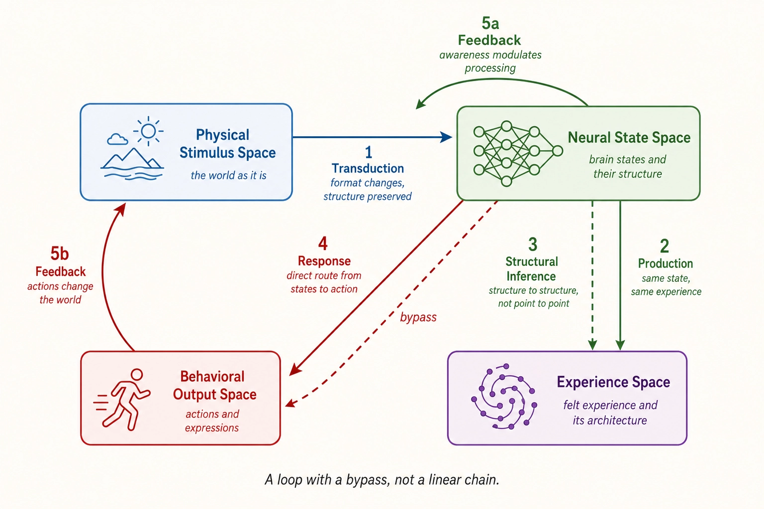
Five mappings describe how information flows between the four spaces. The full picture is a loop with a bypass, not a linear chain. This section defines each mapping’s direction, nature, and key properties. It does not describe how Khozai implements these mappings computationally (that is Sections 4 and 5) or where the mappings break down at the boundaries of the framework (that is Section 6).
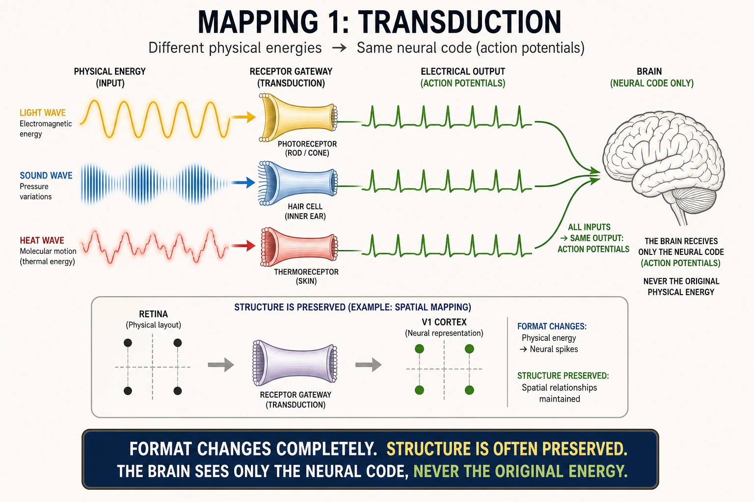
3.1. Mapping 1 - Transduction
From: Physical Stimulus Space to Neural State Space
Nature: Point to point. State-dependent: the same stimulus produces different neural responses depending on the brain’s current configuration. The mapping is (Stimulus x Current Neural State) to New Neural State. Grounded in Premise 2 (receptors transduce physical energy into neural signals).
Key property: The physical format changes completely at the receptor boundary. Electromagnetic radiation becomes action potentials (brief electrical signals that neurons use to communicate). Pressure waves become action potentials. All sensory systems share this property: regardless of the physical energy transduced, the output is the same currency: action potentials whose information is carried by firing rate and temporal pattern, not by the nature of the original stimulus (Kandel et al., 2013 [26]). However, while the format changes, structural relationships are often preserved: V1’s topographic map (a spatial layout in the brain that mirrors the spatial layout of the retina) preserves spatial relationships, and the cochlea’s tonotopic map (a frequency layout where neighboring cells respond to neighboring pitches) preserves frequency relationships. What is radical is the format conversion (photons to electrochemistry), not the destruction of all structure. The brain cannot access the original physical energy - only the neural code that represents it.
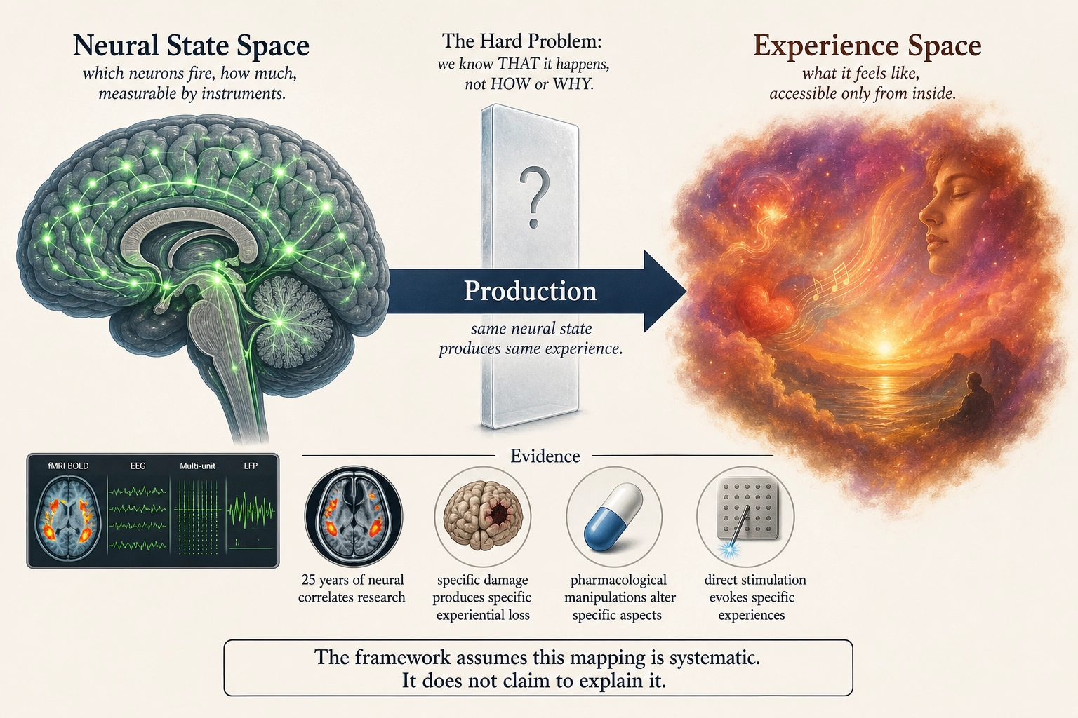
3.2. Mapping 2 - Production
From: Neural State Space to Experience Space
Nature: Point to point. Observed, specific, and graded (Premise 5).
The supervenience assumption. The framework treats this mapping as a function: at the relevant level of neural description, the same neural state gives rise to the same experience. This assumption is known in philosophy of mind as nomological supervenience [13] - the principle that mental states are determined by brain states given the laws of nature. Four lines of empirical evidence support it: (1) the neuroscientist Christof Koch et al. (2016) [14] reviewed 25 years of neural correlates of consciousness research and found that every identified NCC follows a consistent pattern - specific neural states correspond to specific conscious experiences, with no established counterexample. (2) Lesion-deficit correspondences: specific structural damage produces specific experiential loss (the evidence behind Premise 5). (3) Pharmacological manipulations reliably alter specific aspects of experience: anesthetics abolish consciousness dose-dependently (Alkire, Hudetz & Tononi 2008 [15]), dopamine depletion eliminates wanting while preserving liking in rodents (Berridge & Robinson 1998 [8]). (4) Direct cortical stimulation evokes specific experiences: Penfield and Boldrey (1937) [9] mapped motor and sensory responses across hundreds of patients.
This assumption does not, however, resolve the explanatory gap between neural descriptions and phenomenal experience (the philosopher David Chalmers, 1995 [12]; the philosopher Joseph Levine, 1983 [16]). It does not explain WHY a particular pattern of neural activity feels like something - that is the hard problem of consciousness, and it remains unsolved. Among philosophers, the 2020 PhilPapers survey [17] found that roughly 52% accept or lean toward physicalism about the mind - a bare majority, not a consensus. Among working neuroscientists, no comparable survey exists, but the assumption is standard practice: experiments across the field are designed as though brain states determine mental states, even when the metaphysical question is left open. the philosopher Marco Masi (2023) [18], reviewing the relationship between mind-brain identity theory and neuroscientific methodology, describes this as the operational default of the discipline - adopted because it generates testable predictions, not because the philosophical question is settled.
The framework needs this assumption because without it, there is no systematic relationship between neural activity and what a person feels, and the entire project of predicting experience from brain state becomes incoherent. It adopts the nomological form (same neural state, same experience, given our laws of nature) rather than the stronger metaphysical form (same in all possible worlds), which remains contested.
Key property: Covers both Scope A (structure) and Scope B (content) of Experience Space, but we can only characterize Scope A through Structural Inference (Mapping 3).
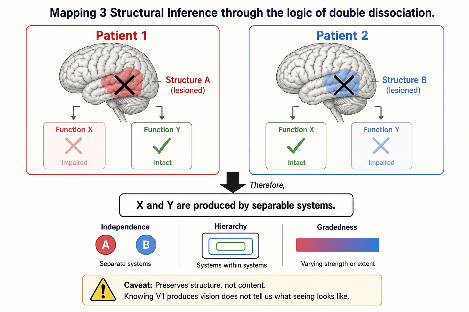
3.3. Mapping 3 - Structural Inference
From: Neural State Space Architecture to Experience Space Architecture
Nature: Structure to structure, NOT point to point. This mapping derives the ARCHITECTURE of Experience Space from the architecture of Neural State Space. It is enabled by Premise 5 and is the mapping the framework actually uses. The formal logic underlying this inference - that if two functions dissociate after neural damage, the systems producing them must be separable - was established by the neuropsychologist Tim Shallice (1988) [27] as the methodological foundation of cognitive neuropsychology.
Limits of the dissociation method. This logic has real critics. the psychologists John Dunn and Kim Kirsner (1988) [33] argued that a single underlying system with different processing demands can mimic both single and double dissociations, and that the assumption of selective influence required for the inference is generally difficult to verify. The framework addresses this in two ways. First, it requires double dissociation as the gold standard (Tool 1), not single dissociation, which raises the evidentiary bar. Second, it treats inferred independence as an empirical hypothesis subject to the Consistency Test (Tool 13) and revision - not as a proven fact. If a claimed dissociation later fails to replicate or turns out to reflect task difficulty rather than separable systems, the affected dimension is reclassified. The method has been the dominant approach for inferring mental structure from neural evidence since its formalization by Shallice (1988) [27], and no alternative method (computational modeling, information-theoretic analysis, convergent multi-method evidence) has replaced it for this specific purpose - establishing which aspects of experience are separable. But it is not infallible, and the framework is designed to correct errors it produces.
What it preserves:
- Independence - if two neural systems are dissociable, the experiential dimensions they produce are independent.
- Hierarchy - if neural processing is nested, experiential dimensions are nested.
- Gradedness - if neural output varies continuously, experiential dimensions vary continuously.
What it does NOT preserve: Content (qualia) - knowing THAT the brainstem reticular activating system (the network of brainstem nuclei that gates whether the cortex is online at all) produces an experiential dimension does not tell us WHAT alertness feels like.
What it does NOT guarantee: Completeness - can only infer experiential structure for neural systems that have been identified and tested. Undiscovered systems mean undiscovered dimensions.
3.4. Mapping 4 - Response
From: Neural State Space to Behavioral Output Space
Nature: Point to point. Probabilistic, not deterministic: the same neural state can produce different behaviors depending on context. Can bypass Experience Space entirely - spinal reflexes, blindsight, and implicit processing produce behavior without corresponding conscious experience. Blindsight, documented extensively by the neuropsychologist Lawrence Weiskrantz (1986) [28], is the clearest demonstration: patients with V1 destruction report no visual experience yet respond accurately to visual stimuli (reaching toward objects, discriminating orientation) when forced to guess - behavioral output driven by neural processing that never entered conscious awareness.
Key implication: Not all behavioral output that Khozai measures was produced through conscious experience. Some stimulus-behavior correlations may reflect unconscious neural processing that never entered Experience Space.
3.5. Mapping 5 - Feedback Loops
Two feedback pathways close the loop:
- Experience to Neural State Space: Conscious awareness modulates subsequent neural processing. Noticing you are anxious changes your neural state. Attending to a stimulus changes how it is processed - the neuroscientists Robert Desimone and John Duncan (1995) [29] demonstrated that top-down attentional signals reshape neural activity in early visual cortex, with attended stimuli producing stronger responses and unattended stimuli suppressed through competitive inhibition.
- Behavioral Output to Physical Stimulus Space: Actions change the physical world, producing new stimuli. Scrolling produces a new video. Speaking produces sound waves. Moving changes visual input. The organism is not a passive receiver: its behavior continuously shapes its own stimulus environment.
Full picture: Physical Stimulus to Neural State to Experience (parallel output) + Behavioral Output (can bypass experience). Experience feeds back to Neural State. Behavior feeds back to Physical Stimulus. A loop, not a chain.
The framework now has structure (premises), domains (spaces), and flow (mappings). The next question: what specific measurements does Khozai compute within these spaces?
4. Vectors
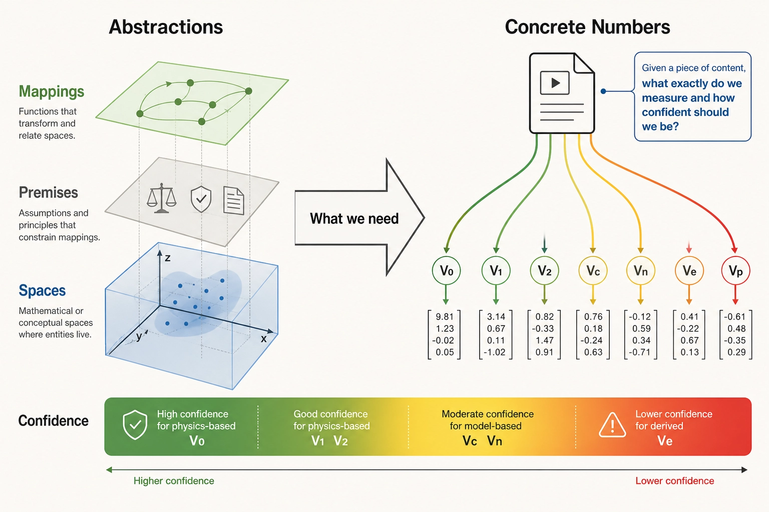
The framework defined four spaces (Physical Stimulus, Neural State, Experience, Behavioral Output) and the mappings between them. But spaces and mappings are abstractions. To do anything useful - to predict, measure, compare, or learn - we need concrete numbers attached to concrete content. That is what vectors are: the specific quantities that Khozai computes or collects for each piece of content.
The goal of this section is to answer a practical question: given a piece of content (a video, an image, an audio clip), what exactly do we measure, and how confident should we be in each measurement? Some vectors are computed from physics with no model uncertainty (V0, V1, V2). Others are approximations produced by AI models, and their quality depends on how good those models are - which varies dramatically by content type. The evidence presented below establishes, modality by modality, where these approximations are strong, where they are weak, and where the gaps remain.
This section defines what each vector is, which space it belongs to, and how strong the evidence is for each. It does not define how each vector is computed: that is Chapter 5’s job.
4.1. Architecture Overview
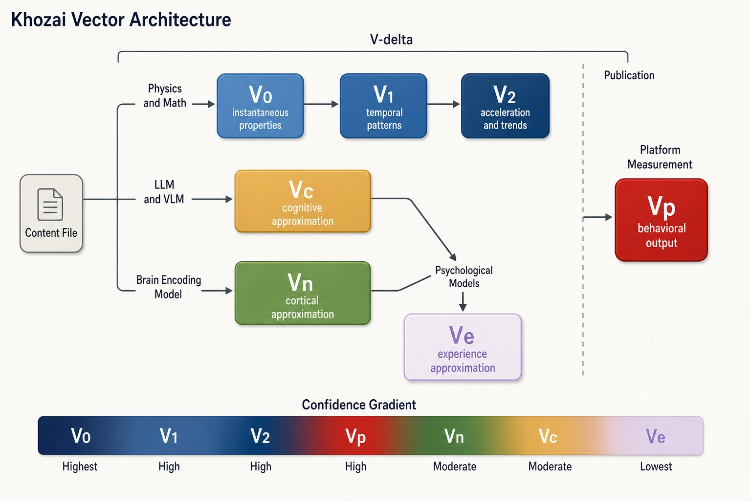
Three parallel extraction paths from the content file, plus derived experience approximation and post-publish measurement:
| Vector | Space | Input | Method | What It Answers |
|---|---|---|---|---|
| V0 | Physical Stimulus | Content file | Physics + math | What is physically in this content? |
| V1 | Physical Stimulus | V0 | Signal processing on V0 over time | What first-order temporal patterns exist? |
| V2 | Physical Stimulus | V1 | Second-order derivations from V1 | What acceleration/momentum/trend patterns exist? |
| Vc | Neural State (cognitive approximation) | Content file | LLM for text, VLM for visual content (evidence strength varies by modality - see below) | What cognitive processing does the content likely elicit? |
| Vn | Neural State (cortical approximation) | Content file | Brain encoding model applied to content (see limitations below) | What cortical activation does the content likely produce? |
| Ve | Experience (derived approximation) | Vc + Vn | Psychological mapping models applied to neural state vectors (see evidence and limitations below) | What experiential state does the content likely produce? |
| Vp | Behavioral Output | Platform | Direct measurement post-publish | What did viewers do? |
Key architectural principle: V0, Vc, and Vn are siblings - all extracted directly from the content file, independently, in parallel. V1 and V2 derive sequentially from V0. Ve is a child of Vc and Vn, projecting their outputs into experiential dimensions. This parallel design matters: Vc and Vn process the full content file through models trained on human data, so if there is a physically measurable property we forgot to include in V0, it is lost in the V0-V1-V2 chain but might still be captured by Vc or Vn. Ve then asks: given what the brain likely computes (Vc) and how cortex likely activates (Vn), what does the person likely experience?
Table 4.1b. Vector space assignments and evidence requirements.
| Vector | Space | Evidence Basis | Key Limitation |
|---|---|---|---|
| V0 | Physical Stimulus | Physics/math - no perceptual model needed | Only captures properties we define; can miss what we forget |
| V1, V2 | Physical Stimulus | Derived from V0 via signal processing | Inherits V0’s completeness limitations |
| Vc | Neural State (cognitive approx.) | Understanding benchmarks (Table 4.2) + brain-similarity studies (Table 4.3) | Approximation quality varies by modality (text > images > audio > video) |
| Vn | Neural State (cortical approx.) | Brain encoding models trained on fMRI data | Inherits fMRI limitations: ~1-2mm spatial, ~1-2s temporal resolution |
| Ve | Experience (derived approx.) | Psychological mapping models: dimensional affect (Russell 1980, Fontaine 2007), constructionist theory (Barrett 2017), neural signatures (Chang 2015, Lee 2024) | Derived from Vc + Vn - inherits their limitations plus uncertainty in psychological mapping models |
| Vp | Behavioral Output | Direct platform measurement post-publish | Only captures measured behaviors; unmeasured responses are invisible |
| V-delta | Same as parent vector | Subtraction of reference from variant | Meaning of subtraction varies by vector type (Chapter 5) |
4.2. V0, V1, V2: Physical Stimulus Vectors
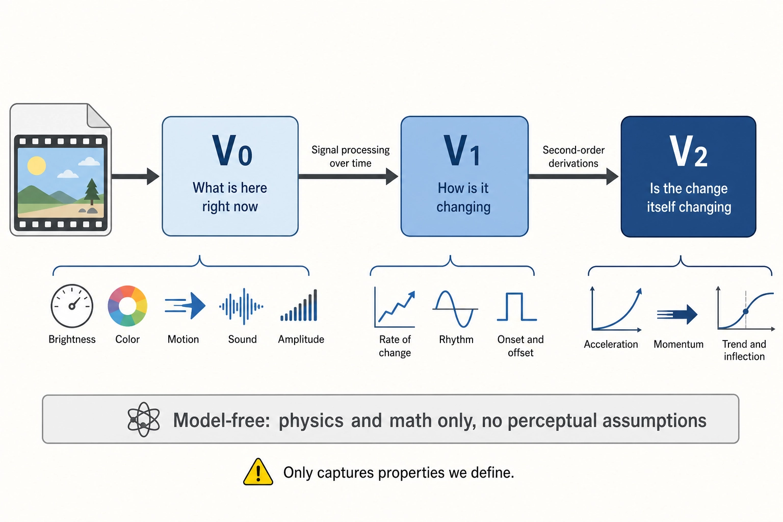
V0 captures what is physically in the content at each instant: luminance, color, motion, audio frequency, amplitude. It is computed with physics and math only - no perceptual model, no assumptions about how a viewer processes it. V1 applies signal processing to V0 over time, extracting first-order temporal patterns (rates of change, rhythms, onset/offset timing). V2 applies second-order derivations to V1, extracting acceleration, momentum, and trend patterns. The V0-V1-V2 chain is the only part of the architecture with no model uncertainty: these are direct measurements of physical properties. Their limitation is completeness - V0 only captures properties we define. If we forget to include a physically measurable property, it is lost in the entire chain.
4.3. Vc: The Cognitive Approximation Vector
What Vc captures. Vc approximates the computational level of neural processing: what semantic content, concepts, and relationships the brain extracts from content. The distinction between Vc and Vn maps onto the computational neuroscientist David Marr’s (1982) [35] framework for analyzing information processing systems: the computational level (WHAT is being computed) versus the implementation level (WHAT HARDWARE does the computing). Vc is the computational level; Vn (Section 4.4) is the implementation level.
Why Vc belongs in Neural State Space. Semantic meaning is not a disembodied abstraction: it is physically encoded in neural firing patterns. This is empirically established. The computational neuroscientist Tom Mitchell and colleagues (2008) [38] demonstrated that fMRI activation patterns for concrete nouns can be predicted from text corpus co-occurrence statistics: the statistical structure in language reflects the statistical structure in neural semantic representations. The neuroscientist Alexander Huth and colleagues (2016) [37] mapped these representations across the entire cortex during naturalistic story listening, revealing continuous semantic maps that tile most of the cortical surface. Meaning is distributed neural activity.
The convergence between LLM representations and neural representations strengthens this placement. The computational neuroscientists Charlotte Caucheteux and Jean-Remi King (2022) [81] showed that middle layers of LLMs best predict brain recordings during natural language processing, suggesting that LLMs and brains partially converge on similar representational structures. The neuroscientist Ariel Goldstein and colleagues (2022) [84] demonstrated shared computational principles between human brains and deep language models: both systems use context to predict upcoming words, and the degree of neural alignment tracks the model’s next-word prediction accuracy. The computational neuroscientist Martin Schrimpf and colleagues (2021) [36] reported that the neural architecture of language models converges on predictive processing - the same principle the brain uses - though this claim has been challenged (Section 4.4). Together, these findings support placing LLM representations in Neural State Space: the representations are not identical to neural activity, but they occupy a demonstrably overlapping region of the same computational landscape.
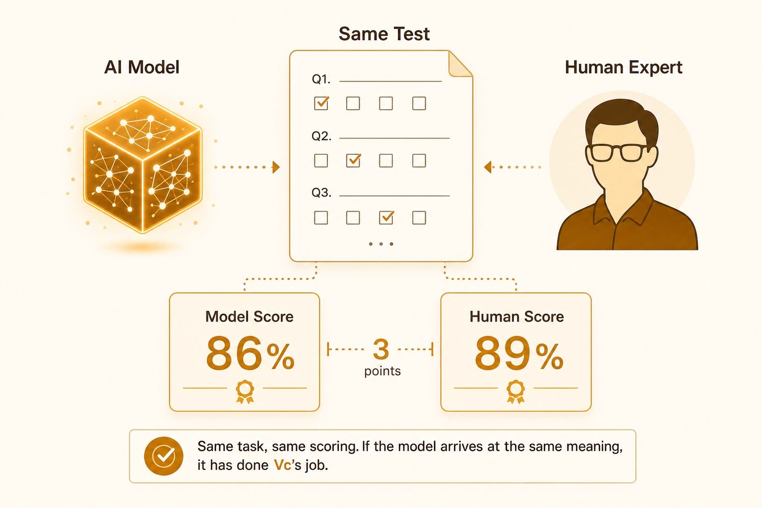
How Vc is evaluated. Vc’s primary evidence is understanding benchmarks - the same approach as a school exam. Give the model and a human expert the same task (describe this image, answer this question about the video, transcribe this audio) and compare their scores. The human baseline is expert performance on the same test. A model that scores 86% on a test where humans score 89% has a 3-point understanding gap. This is the right test for Vc because Vc’s job is to capture what the brain extracts from content - if the model arrives at the same meaning, it has done Vc’s job regardless of how it got there internally.
The evidence is organized by modality because the quality of Vc’s approximation varies dramatically depending on what type of content is being processed.
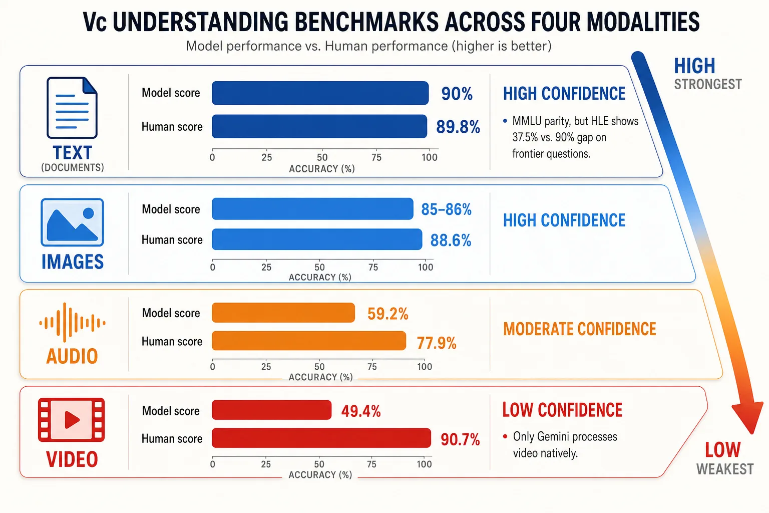
Text. The evidence for text depends on which benchmark you trust. On MMLU (Hendrycks et al., 2021 [78]), a 57-task benchmark spanning STEM, humanities, and social sciences, as of early 2026, frontier LLMs score ~90% against a human expert baseline of ~89.8% - effective parity. On GPQA (Rein et al., 2024 [79]), a set of 448 graduate-level science questions where PhD domain experts scored 65%, frontier models reach ~94% - far exceeding the experts who wrote the questions. But Humanity’s Last Exam (Phan et al., 2026 [80]), published in Nature, was designed to resist this pattern: 2,500 questions authored by over 1,000 domain experts across mathematics, humanities, and natural sciences. Human experts score ~90% in their own domains; the best model scores 37.5% without tools. The picture is benchmark-dependent: models have saturated established tests but still fall far short on questions specifically designed to probe the boundaries of expert knowledge. For Vc’s purposes, the relevant question is whether models extract the same semantic content humans extract from typical text - and on that question, the established benchmarks say yes.
Images. The vision researcher Xiaomin Yue and colleagues (2024) [47] introduced MMMU, a benchmark of 11,500 questions requiring expert-level visual reasoning across 30 subjects. As of early 2026, frontier VLMs score 85-86% versus human experts at 88.6% - a gap of roughly 3 points. Jiang et al. (2025) [48] found that frontier VLMs match human annotators on detailed image captioning, the first time a model reached parity on this task.
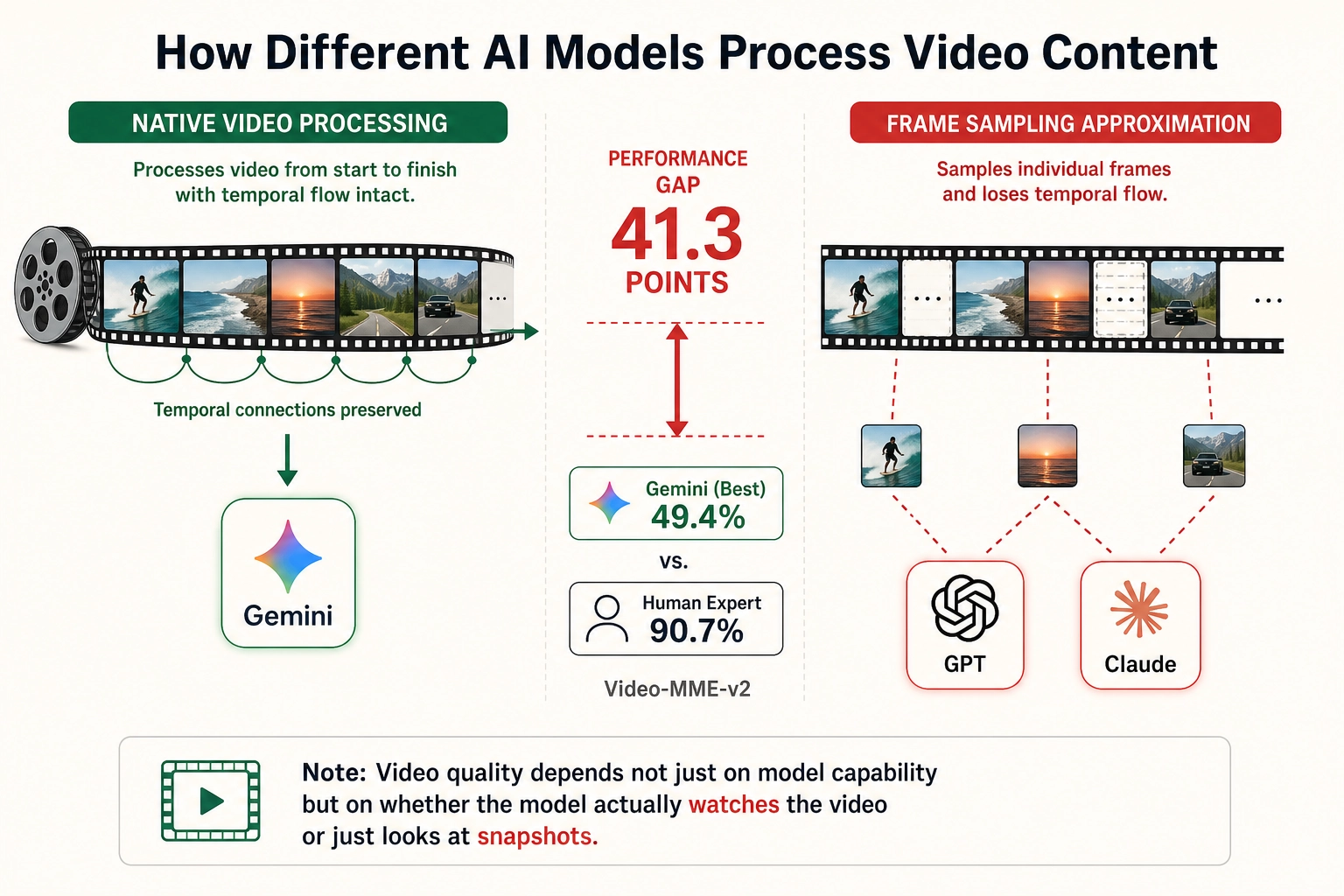
Video. Fu et al. (2025) [49] benchmarked models on Video-MME, a test of video understanding across durations and content types: frontier models score 75-85%. But the harder Video-MME-v2 (Fu et al., 2026 [50]) reveals a much larger gap: the best model (Gemini-3-Pro) scores 49.4% versus human experts at 90.7%.
A structural factor explains part of this gap: as of mid-2026, only the Gemini model family processes video natively from start to finish. Other frontier models (GPT-5, Claude) handle images but not video directly - they approximate video understanding by sampling individual frames, losing the temporal flow that the brain processes continuously. Vc’s video quality therefore depends not just on model capability but on whether the model actually watches the video or just looks at snapshots - a choice that Chapter 5 specifies.
Audio. Yang et al. (2024) [54] introduced AIR-Bench, the first comprehensive benchmark for audio-language models, covering speech, environmental sounds, and music. The MMAU-Pro benchmark (Kumar et al., 2025 [82], preprint) tests complex audio reasoning across 49 skills: the best model (Gemini 2.5 Flash) scores 59.2% versus human experts at 77.9% - an 18.7-point gap.
Table 4.2. Vc understanding evidence by modality.
| Modality | Model score vs human expert | Gap | Vc Confidence |
|---|---|---|---|
| Text | MMLU: ~90% vs 89.8% human (Hendrycks 2021 [78]). GPQA: ~94% vs 65% expert (Rein 2024 [79]). But HLE: 37.5% vs ~90% expert (Phan, Nature 2026 [80]) | Parity on established benchmarks; large gap on frontier-difficulty tests | High (for typical content) |
| Images | MMMU: 85-86% vs 88.6% human (Yue 2024 [47]). Captioning: parity (Jiang 2025 [48]) | ~3 points | High |
| Audio | MMAU-Pro: 59.2% vs 77.9% human (Kumar 2025 [82]) | ~19 points | Moderate |
| Video | Video-MME-v2: 49.4% vs 90.7% human (Fu 2026 [50]). Only Gemini processes video natively | ~41 points | Low |
All benchmark scores as of early 2026. AI benchmark numbers age in months - verify against current leaderboards before publication. Vc’s approximation quality follows a clear gradient: text > images > audio > video.
Why the approximation is still imperfect. Even when models understand content correctly, they do not build meaning the way the brain does. The brain constructs semantic representations from sensory experience, a body, emotions, personal memories, and goals - all running simultaneously. The neurolinguists Olaf Hauk, Ingrid Johnsrude, and Friedemann Pulvermuller (2004) [39] showed that simply reading action words activates motor cortex in a body-mapped pattern: “lick” activates face motor areas, “kick” activates leg motor areas. The brain’s representation of “kick” includes the motor program for kicking - meaning grounded in bodily experience. A VLM identifies the kicking action from visual features but has no body to ground it in. (This finding is debated: Mahon and Caramazza (2008) [40] argue the motor activation is a side effect rather than part of the meaning itself. Either way, the brain draws on sources - bodily, emotional, experiential - that current models lack.)
Models also fail differently than humans. They can struggle with tasks humans find easy (spatial reasoning, counting, reading social dynamics) and succeed at tasks humans find hard (recalling obscure facts, processing many images at once). The match is in what is extracted, the semantic content, not in how it is extracted or in which edge cases break.
4.4. Vn: The Cortical Approximation Vector
What Vn captures. Vn approximates the implementation level of neural processing: which cortical regions activate, at what magnitude, in response to content. Where Vc asks “what does the brain extract from this content?”, Vn asks “which parts of the brain light up, and how much?” Vn is computed by brain encoding models trained on fMRI data.
A different type of evidence: brain similarity. Because Vn targets the implementation level rather than the computational level (Section 4.3), it requires a different evaluation method. Vn is evaluated by comparing a model’s internal processing to actual brain activity measured in a scanner. This answers a different question from Vc’s understanding benchmarks: not whether the model gets the right answer, but whether it organizes information the same way a brain does internally.
How brain-similarity studies work. Researchers show the same content - a sentence, an image, a sound clip - to both an AI model and to human participants lying inside an fMRI scanner. The model produces internal activation patterns (numbers across thousands of artificial neurons in a processing layer); the scanner records blood-flow changes across the brain (a proxy for neural activity, measured across thousands of small volume elements called voxels). These two outputs are in completely different formats - thousands of artificial neuron values versus thousands of brain blood-flow measurements - and cannot be compared directly. Instead, researchers compare the relationships between patterns.
The comparison method: RSA. Show the model 100 images and it produces 100 internal activation patterns. For each pair of images, compute how similar the two patterns are. This gives a 100-by-100 similarity grid: image 1 versus image 2, image 1 versus image 3, and so on. Now show the same 100 images to a person in the scanner, producing 100 brain activation patterns, and build the same kind of similarity grid. The test is whether the two grids match. If the model’s grid says “a cat photo and a dog photo produce similar internal patterns, but both are very different from a car photo,” and the brain’s grid says the same thing, then the two systems organize information in similar ways - even though one runs on silicon and the other on neurons. This comparison is called representational similarity analysis, or RSA (Kriegeskorte, Mur & Bandettini, 2008 [73]). RSA is one of the most widely used methods in computational neuroscience (over 3,000 citations as of 2025) and the standard tool for comparing representations across different systems.
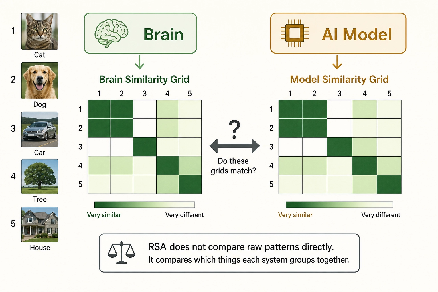
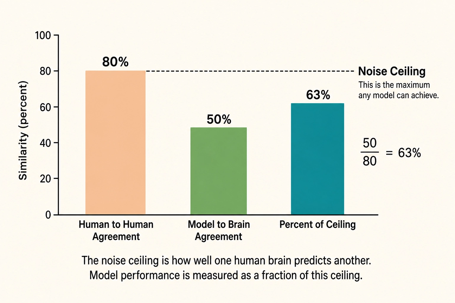
The human baseline for brain similarity is the noise ceiling: how well one person’s brain patterns predict another person’s brain patterns for the same content. If brain-to-brain agreement is 80%, and model-to-brain agreement is 50%, the model captures about 63% of what is consistent across human brains.
An important caveat: RSA reveals whether two systems organize information in similar ways; it does not prove they compute it the same way (Dujmovic et al., 2022 [74], preprint). A model and a brain can group cats with dogs and away from cars for entirely different internal reasons.
The evidence is organized by modality because brain similarity, like understanding, varies dramatically by content type.
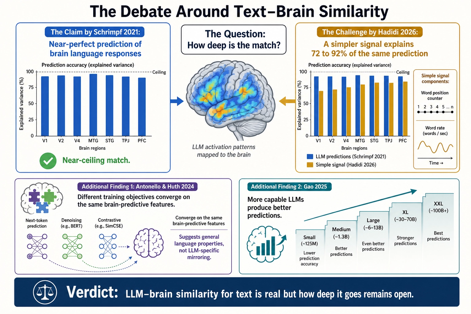
Text. Schrimpf et al. (2021) [36] tested whether LLM internal patterns match brain responses by using LLM activations to predict fMRI scans word by word. They reported a near-perfect match: LLMs predicted almost all of the brain’s language responses that any model could ever predict. But this finding is now contested. The computational neuroscientist Hamid Hadidi and colleagues (2026) [51] showed that much simpler signals - just the position of a word in a sentence and how fast words appear - predict brain responses almost as well as the full LLM. If a simple word counter performs nearly as well as a sophisticated language model, the apparent match may reflect shallow statistical patterns rather than deep understanding. Antonello and Huth (2024) [52] showed that models trained with completely different objectives discover the same brain-predictive features, suggesting the alignment comes from general properties of language, not from LLMs specifically mirroring the brain. LLM-brain similarity for text is real - Gao et al. (2025) [53] confirmed that more capable LLMs produce better brain predictions - but how deep it goes remains open.
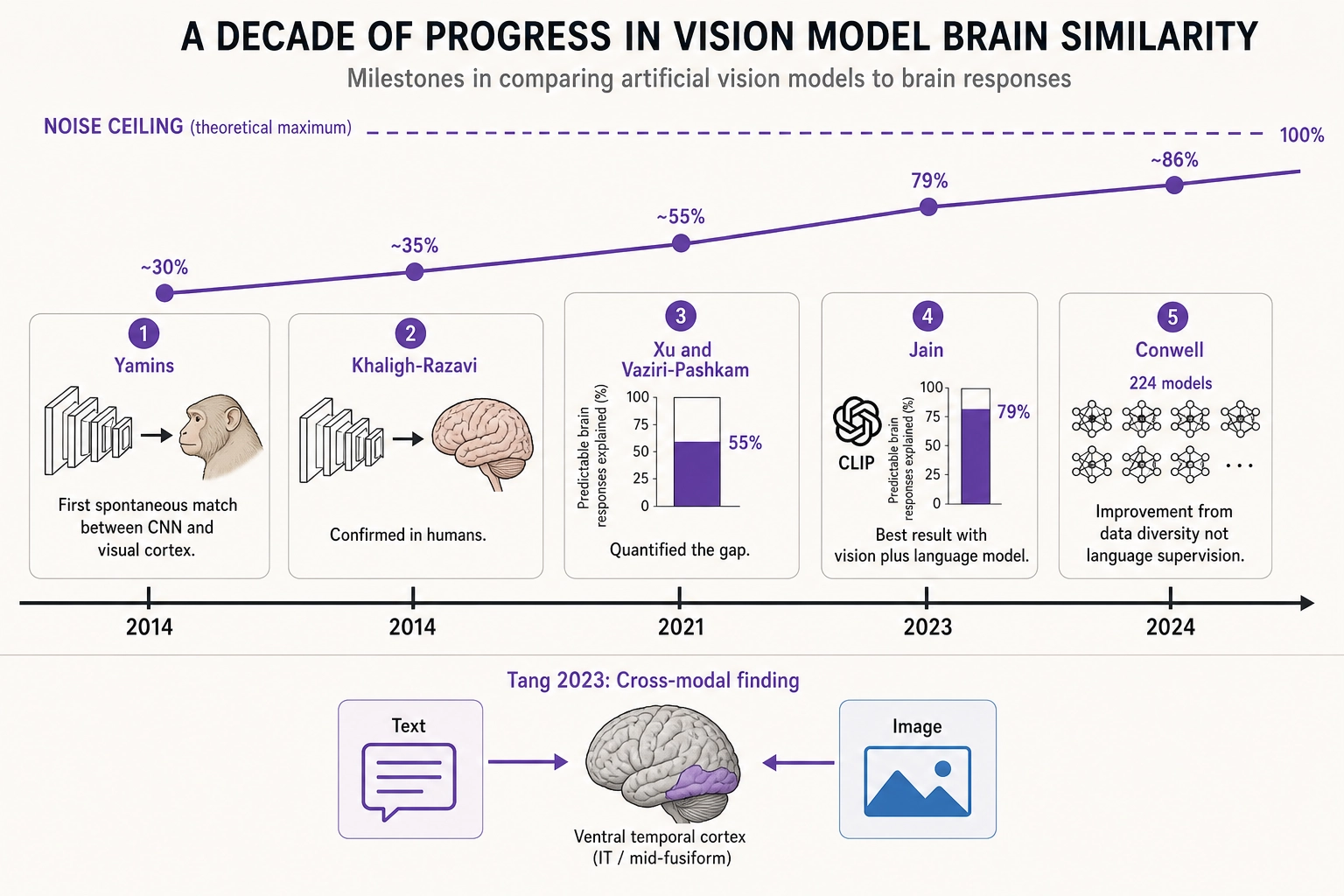
Images. The field has tracked how well vision models’ internal layers predict brain responses in visual cortex. The results have improved over a decade but remain below a perfect match:
| Study | Model Type | Brain Region | How much brain activity the model predicts | Challenge |
|---|---|---|---|---|
| Yamins et al. 2014 [41] | CNN (object recognition) | Macaque V4 and IT cortex | First demonstration of spontaneous match | Foundational, but animal data |
| Khaligh-Razavi & Kriegeskorte 2014 [42] | CNN (supervised) | Human IT cortex | Confirmed match in humans | - |
| Xu & Vaziri-Pashkam 2021 [43] | Best CNNs | Human higher visual cortex | 50-60% of predictable brain responses | Quantifies the gap: models miss 40-50% |
| Jain et al. 2023 [44] | CLIP (vision + language) | Human high-level visual cortex | Up to 79% | Best result so far |
| Conwell et al. 2024 [45] | 224 models compared | Human visual cortex | Varies by model | The improvement comes from training data diversity, not language supervision |
Tang et al. (2023) [46] added a cross-modal finding: models trained on one modality (e.g., text) can predict brain responses to another (e.g., images) in regions that represent conceptual meaning - evidence that the brain uses shared semantic representations across senses.
Video. Video brain similarity has three early studies (all 2025), none yet replicated. An important caveat: the models tested are not the same as the VLMs evaluated in Vc’s understanding benchmarks. The first two studies test video classification models and a video-language pretraining model using RSA; the third tests instruction-tuned VLMs but uses encoding models (regression) rather than RSA, so its results are not directly comparable to the RSA percentages reported for images and text.
| Study | What it showed | Limitation |
|---|---|---|
| Sartzetaki et al. 2025 [75] | RSA comparison of 99 video and image models to fMRI. Video models outperform image models in early visual cortex (motion processing), but in semantic regions the classification task matters more than temporal architecture | Tests video classifiers (SlowFast, MViT), not VLMs |
| Fu et al. 2025 [76] (reviewed preprint) | RSA comparison of VALOR (video-audio-language model) to fMRI. VALOR outperformed all unimodal and static models in semantic brain regions (middle temporal gyrus, angular gyrus, posterior cingulate) | VALOR is a pretraining model, not an instruction-tuned VLM |
| Oota et al. 2025 [77] (preprint) | Encoding model comparison of instruction-tuned VLMs (LLaVA, Qwen-VL) to fMRI during video watching. VLMs outperform non-instruction-tuned models by ~15% and unimodal models by ~20% | Uses regression, not RSA - percentages are not comparable to the RSA figures above |
The pattern is consistent across methods: adding language to a video model improves alignment with semantic brain regions. The specific combination - RSA comparison of VLM internal representations to brain activity during video - remains an open gap.
Audio. Audio follows the same pattern as vision - models predict brain responses better than simple baselines, but fall short of a complete match:
| Study | What it showed | Limitation |
|---|---|---|
| Kell et al. 2018 [55] | A DNN trained on speech and music recognition predicted auditory cortex fMRI responses better than simpler acoustic models, and developed separate speech/music pathways that mirror how auditory cortex is organized | Single model, not replicated at scale |
| Millet et al. 2022 [56] | Wav2Vec 2.0 (a self-supervised speech model) developed an internal hierarchy that maps onto the cortical speech processing hierarchy. Validated on 386 participants - the largest auditory brain-imaging benchmark at the time | Self-supervised model only; not tested with newer audio-language models |
| Tuckute et al. 2023 [57] | Most audio DNNs outpredict simple acoustic baselines. Middle layers predict primary auditory cortex; deep layers predict higher auditory areas | No model approaches a complete match |
| Millet et al. 2024 [58] | Speech models capture acoustic and sound-level structure well but miss the semantic depth found in brain data | Current models are good at “what does this sound like?” but weak at “what does this sound mean?” |
Table 4.3. Brain similarity evidence by modality.
| Modality | Do the model’s internals resemble brain activity? | Status |
|---|---|---|
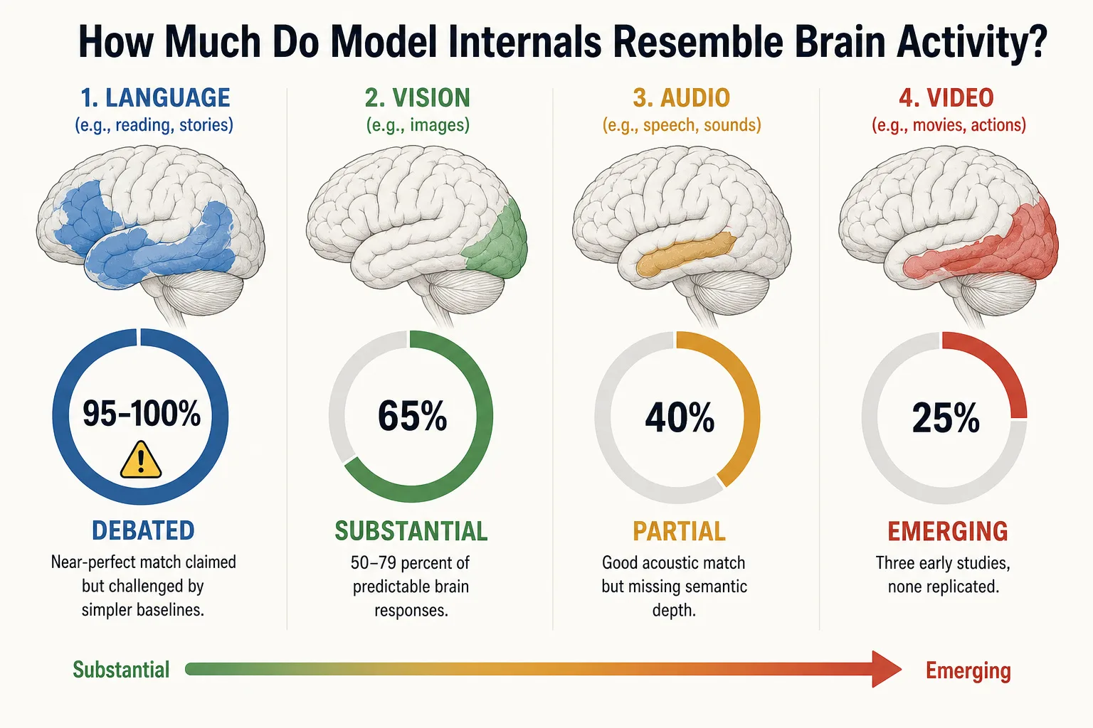
| Text | Real but debated: Schrimpf 2021 [36] claimed near-perfect match, challenged by Hadidi 2026 [51] and Antonello & Huth 2024 [52]. More capable LLMs predict better (Gao 2025 [53]) | Debated |
| Images | 50-79% of predictable brain responses across a decade of RSA studies (Xu & Vaziri-Pashkam 2021 [43] through Jain 2023 [44]). Improvement driven by data diversity, not language supervision (Conwell 2024 [45]) | Substantial |
| Audio | Models beat simple baselines but miss semantic depth (Millet 2024 [58]) | Partial |
| Video | Emerging: three studies (all 2025), none testing VLMs directly. Video classifiers show partial RSA alignment; multimodal models align better in semantic regions; VLMs outperform unimodal models in encoding studies | Emerging |
Brain similarity supports both Vn (directly) and Vc (as secondary evidence). A high brain-similarity score means the model organizes information like the brain does - it does not prove identical computation (Dujmovic et al. 2022 [74]).
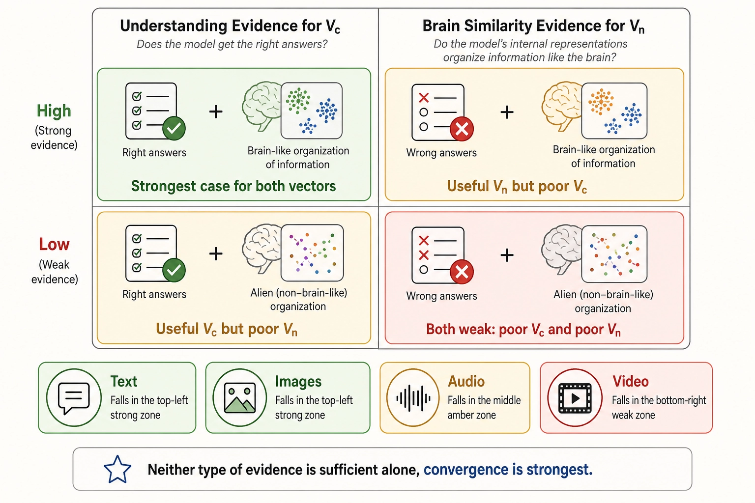
How the two evidence types work together. Tables 4.2 and 4.3 present two different questions about the same modalities, corresponding to the computational versus implementation distinction introduced in Section 4.3. Neither type of evidence is sufficient alone. A model that gets the right answers through alien internal processes (high understanding, low brain similarity) is a useful Vc but a poor Vn. A model whose internals mirror the brain but that fails on tasks (low understanding, high brain similarity) would be a useful Vn but a poor Vc. The strongest case for both vectors is when the two types of evidence converge.
Table 4.4 synthesizes both evidence types into a single view. The numbers in each cell come from different methods and are not on the same scale - understanding scores are exam-style percentages, brain similarity figures come from encoding models (text, images, audio) or RSA (video) - but the confidence gradient is consistent across both columns: text is strongest, video is weakest, and images and audio fall in between.
Table 4.4. Combined evidence for neural state vectors by modality.
| Modality | Model vs Human (Vc evidence) | Brain Similarity (Vn evidence) | Overall Confidence |
|---|---|---|---|
| Text | Parity on MMLU: ~90% vs 89.8% (Hendrycks 2021 [78]). Exceeds PhD experts on GPQA: ~94% vs 65% (Rein 2024 [79]). But 37.5% vs ~90% on Humanity’s Last Exam (Phan, Nature 2026 [80]) | Encoding models predict near-ceiling brain responses (Schrimpf 2021 [36], Caucheteux & King 2022 [81]), but simpler baselines achieve 72-92% of the same prediction (Hadidi 2026 [51]) | High (for typical content) |
| Images | 85-86% vs 88.6% human on MMMU (Yue 2024 [47]); captioning at parity (Jiang 2025 [48]) | Encoding models predict 50-79% of predictable brain responses in visual cortex (Xu & Vaziri-Pashkam 2021 [43], Jain 2023 [44]) | High |
| Audio | 59.2% vs 77.9% human on MMAU-Pro (Kumar 2025 [82]) | Encoding models predict 70-74% of noise ceiling in primary auditory cortex (Kell 2018 [55], Millet 2022 [56]), but miss semantic depth (Millet 2024 [58]) | Moderate |
| Video | 49.4% vs 90.7% human on Video-MME-v2 (Fu 2026 [50]); only Gemini processes video natively | RSA rho (a rank correlation coefficient) of 0.48-0.55 vs ceiling 0.65-0.80, or roughly 60-85% of ceiling (Sartzetaki 2025 [75]). Approximately 25-30% of shared variance if squared - well below the 50-79% encoding model figures for images. Three early studies (all 2025), none yet replicated. No study yet combines VLMs with RSA for video | Low |
Understanding scores are benchmark percentages (model vs human expert on the same test). Brain similarity figures come from encoding model studies (linear regression predicting brain voxel responses) for text, images, and audio, and from RSA (representational similarity analysis comparing similarity matrices) for video. These methods answer related but distinct questions and their numbers are not directly comparable across rows. All figures as of early 2026.
Text is the strongest modality for both vectors. Models match or exceed human expert performance on established language understanding benchmarks - parity on MMLU’s 57 subjects (Hendrycks 2021 [78]), and exceeding PhD experts on graduate-level science questions in GPQA (Rein 2024 [79]). However, Humanity’s Last Exam (Phan et al., Nature 2026 [80]) shows that when questions are specifically designed to probe the frontier of expert knowledge, models score 37.5% versus human experts at ~90%. For Vc’s purposes - extracting semantic content from typical text - the established benchmarks support high confidence. On the brain similarity side, encoding models predict near-ceiling brain responses (Schrimpf 2021 [36], Caucheteux & King 2022 [81]), but simpler signals - word position and word rate - achieve most of the same prediction (Hadidi 2026 [51]), leaving open the question of whether the match reflects genuine linguistic processing or shallow statistical patterns.
Images show a small understanding gap (~3 points on the hardest benchmarks) and substantial brain similarity (up to 79% of predictable responses with vision-language models). The improvement in brain similarity over the past decade has been driven by training data diversity rather than language supervision specifically (Conwell 2024 [45]), and cross-modal studies show that models trained on text can predict brain responses to images in regions that represent conceptual meaning (Tang 2023 [46]).
Audio shows a meaningful understanding gap (~19 points) and partial brain similarity. Models predict acoustic and sound-level brain responses well (70-74% of noise ceiling in primary auditory cortex), but miss the semantic depth found in higher auditory brain regions (Millet 2024 [58]). The gap between acoustic and semantic prediction mirrors the gap between lower and higher auditory cortex, suggesting models capture the “what does this sound like?” but not the “what does this sound mean?”
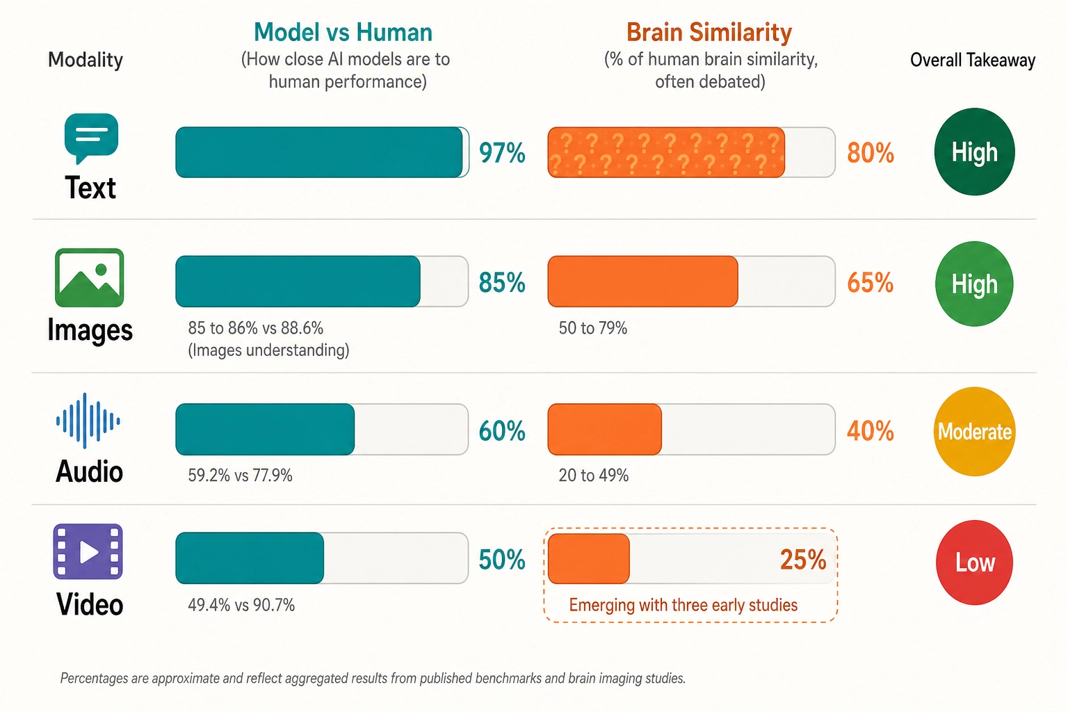
Video is the weakest modality for both vectors. The understanding gap is large (~41 points), partly because most models sample frames rather than processing video natively. Brain similarity evidence is early - three studies from 2025, none yet replicated. The best available numbers come from Sartzetaki et al. (2025) [75], who compared 99 models to fMRI data using RSA: video classifiers achieved rho values of 0.48-0.55 against noise ceilings of 0.65-0.80, depending on brain region. As a ratio, this is roughly 60-85% of ceiling - but rho ratios overstate the comparison with encoding model figures used for other modalities. Squaring rho to approximate shared variance gives roughly 25-30%, well below the 50-79% encoding model figures reported for images. No study yet tests the specific combination of VLMs with RSA for video. The consistent finding across all three video studies is that adding language training improves alignment with semantic brain regions.
The gradient is clear: as content modality moves from text to video, both types of evidence weaken. This does not mean video vectors are useless - it means their approximation quality is lower and should be treated with proportionally more skepticism. Khozai’s correlation engine (Chapter 5) provides a built-in check: if a vector’s predictions consistently fail to track behavioral outcomes (Vp), the framework learns this regardless of what the benchmarks say.
4.5. Ve: The Experience Approximation Vector
What Ve is. Ve is a derived vector that lives in Experience Space. Where Vc and Vn approximate what happens at the computational and implementation levels of neural processing (Section 4.3), Ve approximates what the person experiences - the affective and attentional state that the content likely produces. Ve is not measured directly. It is computed from Vc and Vn using psychological mapping models that translate neural state approximations into experiential dimensions.
Why Ve is an assumption, not a measurement. Experience Space is the one space the framework cannot access from outside (Section 6.4). A point in Experience Space is what it feels like to watch something - subjective, private, accessible only from inside. Every other vector in the architecture is either measured (V0, Vp) or computed from objective models (Vc, Vn). Ve breaks this pattern: it uses psychological theories to infer an experiential point from neural state approximations. This makes Ve the weakest vector in the architecture - an approximation of an approximation, filtered through mapping models that are themselves debated. The framework labels it as such and tracks it precisely because experimentation may reveal whether these inferences hold.
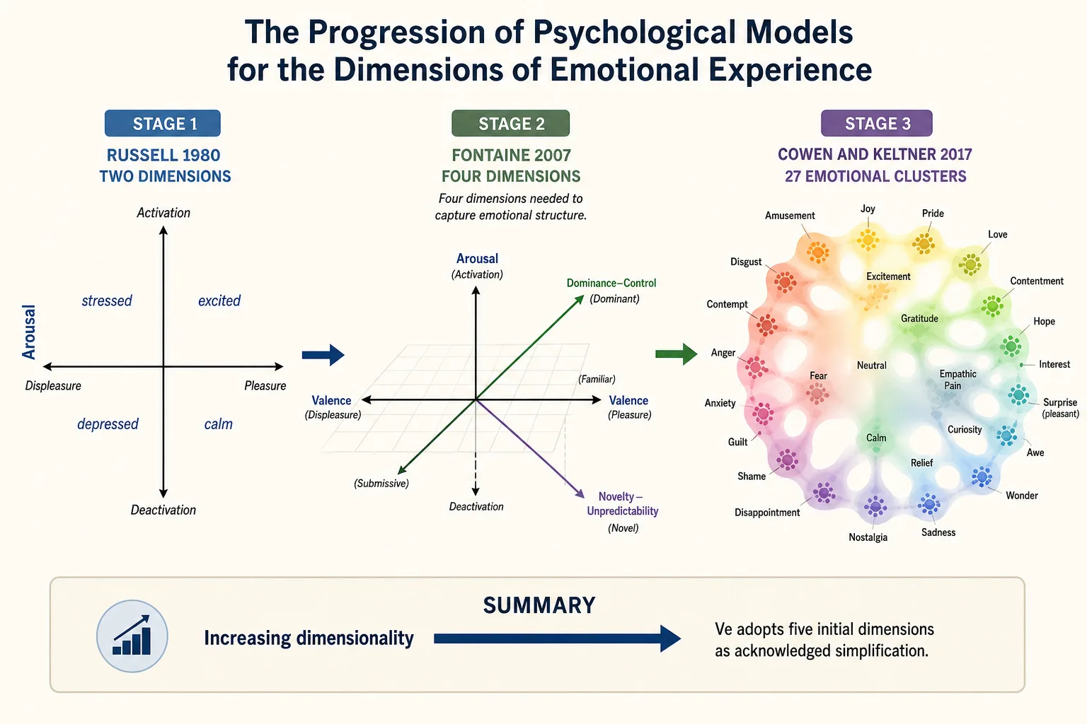
The psychological basis for Ve’s dimensions. What dimensions does experience have? This is itself an empirical question with converging evidence from multiple research traditions.
The psychologist James Russell (1980) [59] established that affective experience can be described in a two-dimensional space defined by valence (pleasure-displeasure) and arousal (activation-deactivation). This two-dimensional model has been replicated across languages, cultures, and methodologies over four decades. Russell (2003) [60] refined this into the concept of “core affect” - a neurophysiological state consciously accessible as a blend of hedonic and arousal values - which provides the theoretical bridge between neural states and experiential dimensions.
However, two dimensions are insufficient. The psychologists Johnny Fontaine, Klaus Scherer, Ethan Roesch, and Phoebe Ellsworth (2007) [61] analyzed 144 emotion features across multiple languages and found that four dimensions are needed to capture the structure of emotional experience: evaluation-pleasantness, potency-control, activation-arousal, and unpredictability-novelty. The third and fourth dimensions (control and novelty) are not reducible to combinations of valence and arousal. This aligns with Scherer and Moors’s (2019) [62] appraisal theory, which models emotion as the output of sequential evaluations of relevance, implications, coping potential, and normative significance - each evaluation producing a distinct experiential dimension.
More recently, the psychologists Alan Cowen and Dacher Keltner (2017) [63] found 27 distinct categories of emotional experience from 2,185 video stimuli, bridged by continuous gradients. This does not eliminate dimensional models but shows that experience has more structure than four axes alone can capture. Ve’s dimensional representation is a simplification - a useful one, but acknowledged as incomplete.
The constructionist basis for Ve = f(Vc, Vn). Why should experience be derivable from Vc and Vn at all? The psychologist Lisa Feldman Barrett’s (2017) [64] theory of constructed emotion provides the strongest theoretical grounding. The theory proposes that emotions are not triggered by stimuli but constructed: the brain makes predictions about the causes of interoceptive signals (internal body signals like heartbeat, gut feelings, breathing rate) and categorizes them using prior conceptual knowledge. In Barrett’s framework, emotional experience emerges from core affect (valence + arousal from these body-state signals) combined with conceptual knowledge (from past experience and cultural learning). This maps directly onto Ve’s architecture: Vn provides the neural activation patterns (analogous to interoceptive signals), Vc provides the semantic/conceptual content, and Ve is their combination through psychological mapping models. Barrett, Atzil, Bliss-Moreau et al. (2025) [65] updated this theory, emphasizing that signals lack inherent emotional significance - meaning derives from relational ensembles in context. The constructionist account is not unchallenged: Adolphs and Anderson (2018) [66] argue that animal studies support evolutionarily conserved neural circuits for basic emotions, though they acknowledge the role of cognitive construction. The truth likely involves both biological roots and constructive processes - Ve accommodates either view by treating the mapping models as replaceable components.
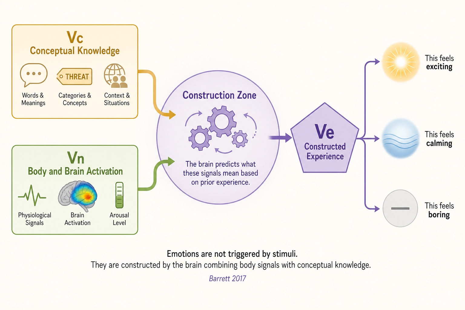
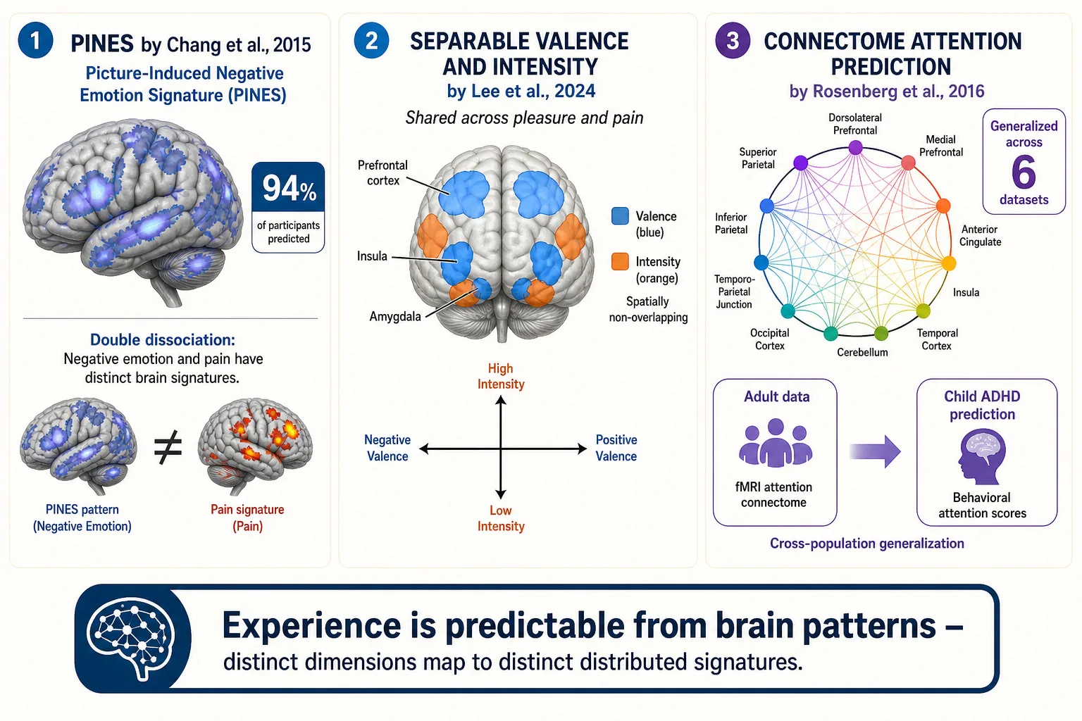
Empirical evidence that experience can be predicted from brain patterns. Ve’s viability depends on whether experiential dimensions can actually be predicted from distributed neural data. Three lines of evidence say yes.
First, Chang, Gianaros, Manuck, Krishnan and Wager (2015) [67] developed PINES (Picture-Induced Negative Emotion Signature), a distributed brain pattern that predicted ratings of negative emotional experience in 94% of participants and classified aversive versus non-aversive pictures with 100% forced-choice accuracy. PINES was specific to negative emotion - it double-dissociated from the Neurologic Pain Signature (Wager et al. 2013 [68]) - demonstrating that distinct experiential dimensions map to distinct distributed brain patterns.
Second, Lee, Lee, Han, Choi, Wager and Woo (2024) [69] identified spatially non-overlapping brain representations for affective valence versus intensity, shared across pleasure and pain. Seven key brain regions - including areas of the prefrontal cortex responsible for value assessment, the insula which tracks body states, and the amygdala which processes emotional significance - encoded these dimensions, with valence correlating with the brain’s emotion and self-reflection networks. This is direct evidence that the brain encodes experiential dimensions in separable, predictable patterns.
Third, for engagement and attention - an experiential dimension beyond affect - Rosenberg, Finn, Scheinost, Papademetris, Shen, Constable and Chun (2016) [70] built a predictive model based on the brain’s complete wiring map (its connectome) that predicted sustained attention from whole-brain functional connectivity. The model generalized across six independent datasets, including predicting ADHD symptoms in children from data collected on adults - evidence that attention/engagement is a stable, predictable experiential dimension encoded in brain connectivity.
A fourth line of evidence extends beyond individual dimensions to continuous experiential states. Tang, LeBel, Jain, and Huth (2023) [83] demonstrated that brain activation patterns recorded with non-invasive fMRI can be decoded into continuous semantic language - reconstructing the meaning of perceived speech from brain recordings alone. This shows that the mapping from neural states to experiential content is structured enough to be inverted: not only can brain patterns predict discrete experiential dimensions (as in the three studies above), but they carry sufficient information to reconstruct the continuous stream of experience itself.
Table 4.5. Ve dimensional foundation: experiential dimensions with empirical grounding.
| Dimension | Foundational Model | Key Evidence | Derivable From | Status |
|---|---|---|---|---|
| Valence (pleasure-displeasure) | Two-dimensional affect model (Russell 1980 [59]) | PINES predicts negative affect in 94% of subjects (Chang et al. 2015 [67]); separable brain signature (Lee et al. 2024 [69]) | Vc (semantic appraisal of content) + Vn (limbic/vmPFC activation patterns) | Well-grounded: 40+ years of dimensional models, confirmed by neural signature research |
| Arousal (activation-deactivation) | Two-dimensional affect model (Russell 1980 [59]) | Separable from valence in brain patterns (Lee et al. 2024 [69]); rooted in internal body-state monitoring (Barrett & Simmons 2015 [71]) | Vn (autonomic-related cortical patterns) + Vc (content intensity features) | Well-grounded: distinct neural basis from valence, interoceptive predictive account |
| Dominance/control | Four-factor model (Fontaine et al. 2007 [61]) | Appraisal component: coping potential (Scherer & Moors 2019 [62]) | Vc (semantic appraisal of agency, threat, controllability) | Moderate: well-established in appraisal theory, less directly mapped to brain patterns |
| Novelty/unpredictability | Four-factor model (Fontaine et al. 2007 [61]) | Linked to prediction error (Joffily & Coricelli 2013 [72]): the brain tracks how much reality deviates from expectations; appraisal component (Scherer & Moors 2019 [62]) | Vc (semantic novelty relative to context) + Vn (prediction error signals) | Moderate: computationally formalizable, but experiential mapping is indirect |
| Engagement/attention | Sustained attention model (Rosenberg et al. 2016 [70]) | Generalized across 6 datasets; predicts attention from brain connectivity | Vc (content complexity, narrative structure) + Vn (front-and-top-of-brain attention network activation) | Emerging: strong neural predictability, but mapping from content features is less validated |
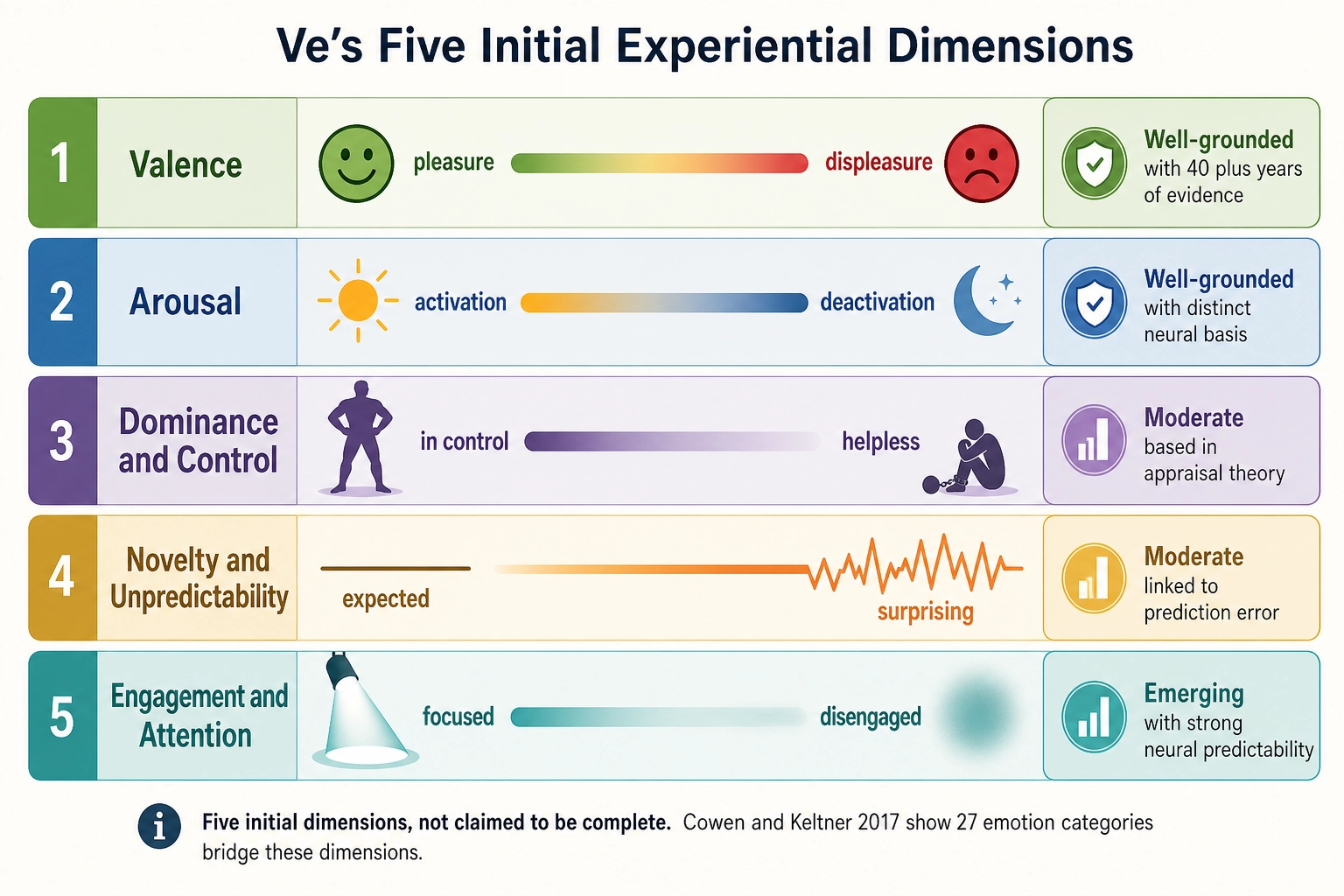
These five dimensions are Ve’s initial operating set. The list is not claimed to be complete - Cowen & Keltner (2017) [63] show that 27 emotion categories bridge these dimensions, and additional dimensions (aesthetic appreciation, social evaluation, temporal anticipation) may prove necessary. Ve’s dimensionality is an empirical question that Khozai’s correlation engine can help answer: if a Ve dimension consistently predicts Vp outcomes that no other vector captures, it earns its place.
Why Ve is worth tracking despite its weakness. Ve is the weakest vector in the architecture. It is derived, not measured. Its mapping models are debated. Its dimensionality may be incomplete. Why include it?
Because Experience Space exists. The framework’s own premises establish that neural states produce experiential states (Mapping 2), and the framework explicitly acknowledges Experience Space as a real domain with inferable structure (Section 6). Leaving it without a vector means the framework has no computational handle on the space it claims is central to understanding content impact. Ve provides that handle, imperfect, approximate, and honestly labeled as such.
The practical value is in what experimentation reveals. Three outcomes are possible, and all are informative. First, Ve may predict Vp outcomes (viewer behavior) that Vc and Vn alone miss - evidence that the psychological mapping models capture something real beyond what the neural state vectors provide. Second, Ve may align with Vc and Vn predictions, converging on the same result from a different angle - this triangulation strengthens confidence in all three vectors, because three independent approximations agreeing is stronger evidence than any one alone. Third, Ve may add no predictive power and fail to converge - evidence that the experiential mapping is either redundant or wrong, which is itself useful to know. Ve exists to be tested, not trusted.
Table 4.6. Vector confidence gradient.
| Vector | Source | Confidence | Why |
|---|---|---|---|
| V0 | Physics + math | Highest | Direct measurement, no model uncertainty |
| V1, V2 | Derived from V0 | High | Signal processing on exact measurements |
| Vp | Platform measurement | High | Direct behavioral observation, but only captures measured behaviors |
| Vn | Brain encoding model | Moderate | Model-based; inherits fMRI limitations (~1-2mm spatial, ~1-2s temporal) |
| Vc | LLM/VLM | Moderate | Model-based; varies by modality (text strong, video weak - see Table 4.4) |
| Ve | Derived from Vc + Vn via psychology models | Lowest | Approximation of approximations; mapping models themselves debated |
The confidence gradient is not a judgment of importance. Ve may prove to be the most practically valuable vector for predicting content impact - but it carries the most epistemic uncertainty, and the framework is honest about that.
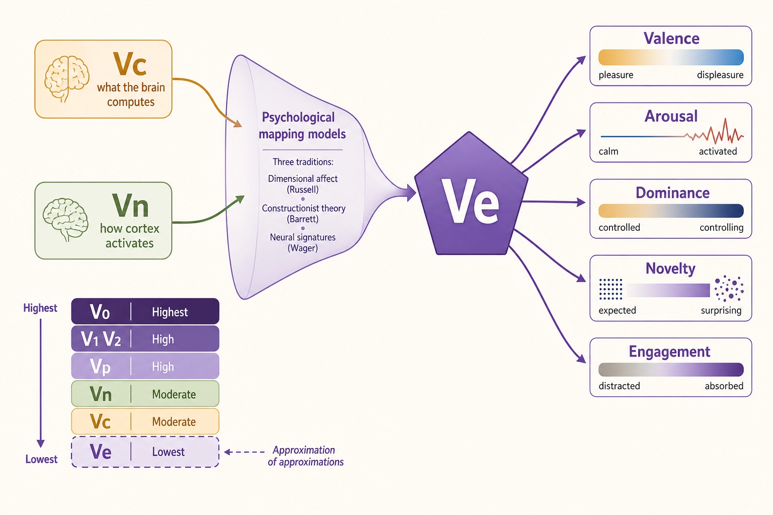
4.6. Vp: The Behavioral Output Vector
Vp is fundamentally different from every other vector in the architecture. V0, Vc, Vn, and Ve are all computed before publication - they are predictions about what the content contains, what the brain will likely do with it, and what the viewer will likely experience. Vp is measured after publication - it records what viewers actually did.
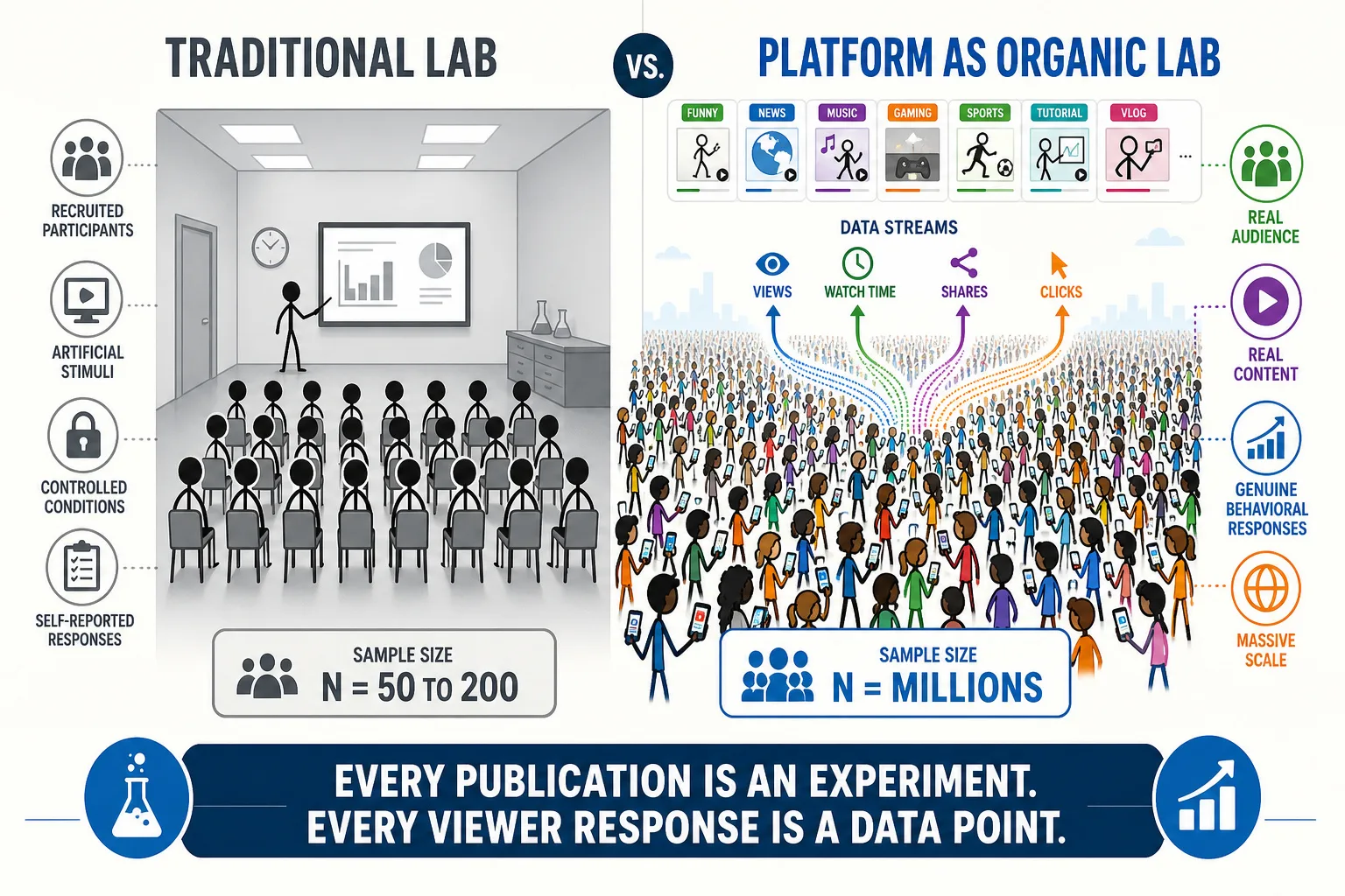
Why publishing is experimenting. Traditional neuroscience and psychology research runs on small samples: tens or hundreds of participants, recruited into a lab, watching stimuli on a screen under controlled conditions. The results are statistically powerful but ecologically limited - people behave differently when they know they are being studied, and lab settings cannot reproduce the context in which people actually encounter content. Content platforms have changed this. Every piece of content published on YouTube, Instagram, TikTok, or any other platform is exposed to real people, in their real environments, making real decisions about whether to watch, stop, share, or scroll past. The platform records those decisions at scale - thousands, millions, sometimes hundreds of millions of behavioral data points per piece of content.
This is an organic laboratory. The “participants” are not recruited - they are the actual audience. The “stimuli” are not artificial - they are the real content. The “responses” are not self-reported in a questionnaire - they are genuine behaviors with real consequences (a viewer who shares a video is putting their social reputation behind it). And the sample sizes are orders of magnitude larger than typical laboratory studies, which rarely exceed a few hundred participants. A single A/B test on a thumbnail - changing one visual element and measuring the click-through difference - can collect more behavioral data points in a day than most psychology studies collect in a year.
This was not possible a generation ago. Before platforms, a content creator could publish a film or a magazine and receive aggregate feedback (box office numbers, subscription counts), but nothing at the granularity of individual viewer behavior over time. The platform era has created an opportunity that did not exist before: every publication is a potential experiment, every viewer response is a data point, and the scale is large enough to detect subtle effects that laboratory studies would miss. Khozai is designed to exploit this opportunity. The entire vector architecture exists so that the framework can ask: given what we predicted about this content (V0, Vc, Vn, Ve), what actually happened when real people encountered it (Vp)?
What Vp measures. Vp captures behavioral outputs from the platform: views, watch time, completion rate, likes, shares, comments, click-through, scroll depth, replays, and any other measurable action. These are direct observations, not model approximations. Vp’s confidence is high for what it measures - a view count is a view count.
The limitation is coverage: Vp only captures behaviors the platform measures. A viewer who watches a video, feels deeply moved, but closes the tab without interacting leaves no trace in Vp. The experiential impact was real but behaviorally invisible. This is one reason Ve matters despite being the weakest vector - it attempts to approximate the experiential states that Vp cannot see.
Table 4.7. What Vp captures and what it misses.
| Vp Captures | Vp Misses |
|---|---|
| Views, impressions, reach | Content seen but not registered (scrolled past too fast) |
| Watch time, completion rate | Attention quality (watching while distracted vs. fully engaged) |
| Likes, shares, saves, comments | Emotional response that produces no action |
| Click-through, link follows | Interest that does not result in a click |
| Replays, rewinds | What specifically triggered the replay |
| Scroll depth, pause points | Why the viewer paused |
| Subscribe/follow after viewing | Long-term attitude change |
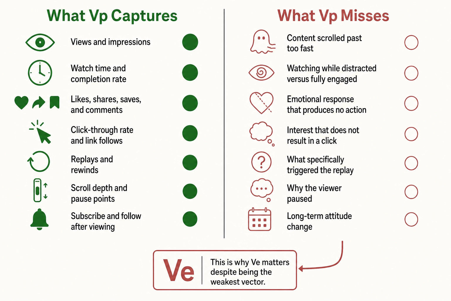
Vp is the ground truth the framework tests against. V0, Vc, Vn, and Ve are predictions; Vp is the outcome. The correlation engine (Chapter 5) measures how well each prediction vector maps to Vp - that is how the framework learns which approximations work and which do not.
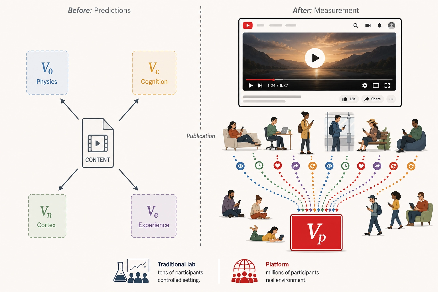
4.7. V-delta: The Difference Vector
V-delta = V_variant minus V_reference, for any vector type. It captures what changed between two versions of content and how that change affected outcomes. V-delta is the foundation of Khozai’s experimental method: controlled perturbation of stimulus properties to observe effects on behavioral outcomes.
For example: take a video thumbnail (reference), change its color grading (variant), and compute V-delta across all vector types. V0-delta shows the physical color difference. Vc-delta shows the semantic shift (if any). Vn-delta shows the predicted change in cortical activation. Ve-delta shows the predicted experiential shift (warmer feeling, higher arousal). Vp-delta shows whether the change actually affected viewer behavior (more clicks, longer watch time). By comparing which prediction deltas best track the behavioral delta, the framework learns which level of description best explains viewer responses.
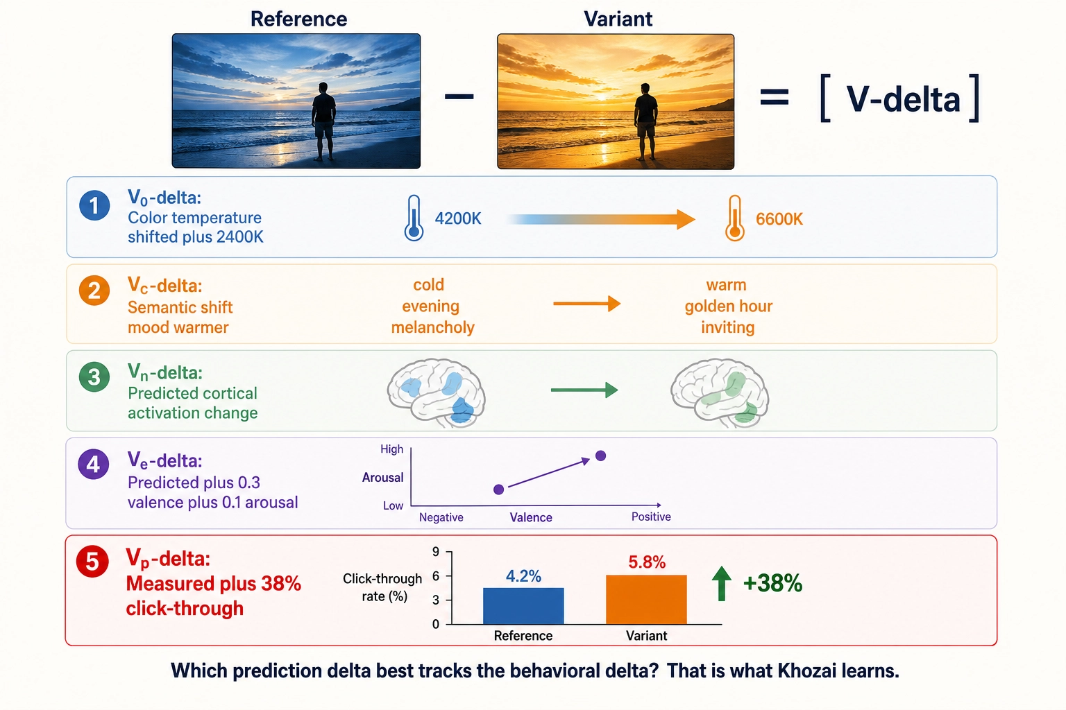
Assumptions and limitations. Several assumptions in this architecture deserve flagging; Chapter 5 examines them in detail.
Vn’s value depends entirely on the quality of the brain encoding model. These models are trained on fMRI data, which has known limitations in spatial resolution (~1-2mm), temporal resolution (~1-2 seconds), and population coverage (typically trained on small samples of Western adults). Vn inherits every limitation of the model that produces it.
Ve inherits every limitation of Vc and Vn, plus the uncertainty of its own psychological mapping models (detailed in Section 4.5).
V-delta (variant minus reference) assumes meaningful subtraction. For V0, this is straightforward: the difference between two luminance values is a real physical quantity. For Vc (LLM embeddings), the meaning of subtraction in high-dimensional embedding space is less clear: what does it mean to “subtract” one semantic interpretation from another? For Vn (predicted activations), subtraction is more defensible since activation values are scalar magnitudes. For Ve (experiential dimensions), subtraction is meaningful along individual dimensions (a valence difference of 0.3) but combining dimensions into a single “experiential distance” requires weighting assumptions that Chapter 5 specifies. The interpretation of V-delta varies by vector type, and Chapter 5 specifies what subtraction means for each.
The computation, properties, and relationships of each vector are defined in Chapter 5. What matters for this chapter is the architecture: which spaces the vectors live in, how they relate to each other, and what questions each one answers.
The framework has premises, spaces, mappings, and measurement objects. The next question: what formal operations let us discover, test, and validate claims within this framework?
5. Reasoning Tools
Thirteen formal operations for discovering, testing, and validating claims within the framework. Each tool has a specific purpose and a defined procedure. This section defines what each tool does and when to use it. It does not apply the tools to specific claims (that is the work of Chapters 4 through 7) or describe how Khozai automates them computationally (that is Chapter 5).
The tools are organized into three groups by function: discovery (finding and verifying experiential dimensions), characterization (classifying and assigning framework components), and validation (ground-truthing against evidence and internal consistency). The tool numbers (1-13) reflect the order in which the framework introduced them during development; the grouping below is by function, not by number, so the numbering within each group is non-sequential.
5.1. Discovery Tools
These five tools find, verify, and organize the dimensions of Experience Space.
Tool 1 - Dissociation Test. Tests independence between two experiential aspects. If altering structure A changes experience X but not Y, and altering structure B changes experience Y but not X, then X and Y are independent dimensions. This two-way demonstration is called a double dissociation - the methodological standard for establishing separability, formalized by Shallice (1988) [27] and discussed with its limitations in Section 3.3. Single dissociation (one direction only) is suggestive but can be explained by difficulty differences. Grounding: follows directly from Premise 5.
Tool 2 - Atomicity Test. Tests whether a candidate dimension is genuinely irreducible. Three sub-tests, ALL of which must pass: (2a) Non-composability - the state cannot be fully expressed as a combination of other states; (2b) Independent variability - the state can change while all other states remain constant, demonstrated through experimental evidence, not just logical argument; (2c) Dedicated hardware - the state maps to neural substrate that is not fully shared with any other state’s substrate.
Tool 3 - Spanning Test. Tests whether the dimension set covers all of Experience Space. Attempt to find an experience that cannot be described as a point using the current dimensions. If found, either a dimension is missing or the resolution is too coarse. Can be falsified (one counter-example) but never proven complete. Confidence increases with diversity and number of failed falsification attempts.
| Tool | Question It Answers | Gold Standard |
|---|---|---|
| 1 - Dissociation | Are X and Y independent dimensions? | Double dissociation (both directions) |
| 2 - Atomicity | Is this dimension genuinely irreducible? | All three sub-tests pass |
| 3 - Spanning | Does the dimension set cover all of Experience Space? | No counter-example found |
Tool 4 - Hierarchy Test. Tests whether dimension B is a child of dimension A. Dimension B is a child of A if and only if eliminating A’s hardware also eliminates B, but eliminating B’s hardware does not eliminate A. Destroying V1 (the primary visual cortex, as introduced in Premise 5) eliminates all vision including color - color is a child of vision. Destroying V4 (the cortical area specialized for color processing, one of the regions downstream from V1) eliminates color but not motion - color and motion are siblings, both children of vision.
Tool 6 - Pattern Verification Test. Tests whether a construct is a pattern across dimensions rather than an atomic dimension. Four steps: (1) Map the construct to specific values across existing dimensions. (2) Test whether altering ONE dimension shifts the experience OUT of the construct. (3) Test whether ALL components are necessary: if removing any single one transforms the experience away from the construct, it is a conjunction. (4) Test for residual: after accounting for all components, is there anything left? If no residual, confirmed as pattern.
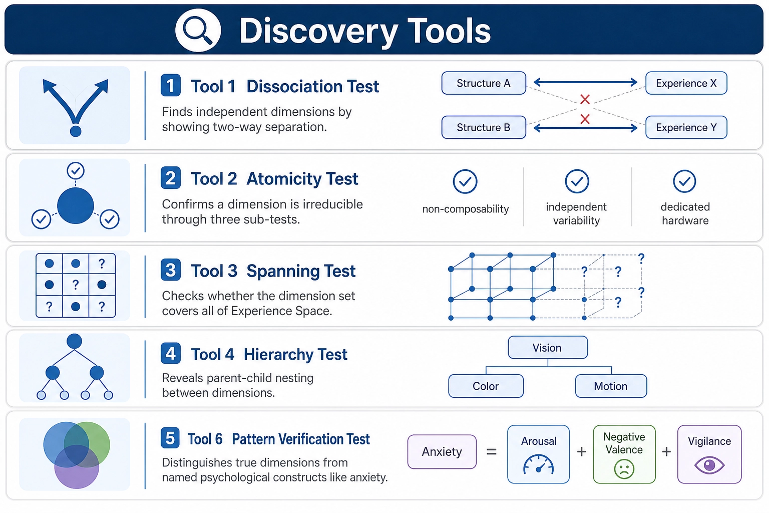
5.2. Characterization Tools
These five tools classify, assign, and trace the components of the framework.
Tool 5 - Classification Test. Determines a neural system’s role: state producer, modulator, or infrastructure. Destroy or disable system S and observe: Does a specific aspect of experience disappear? The system is a state producer. Do existing aspects change in character but none disappear? The system is a modulator. Does processing efficiency degrade but experiential character remain unchanged? The system is infrastructure.
Tool 7 - Resolution Selection Principle. Determines the appropriate resolution for a specific purpose. The appropriate resolution is the coarsest at which no operationally relevant information is lost. For the philosophy: finest resolution. For Khozai’s operational system: the resolution at which experiential differences produce measurable behavioral differences, empirically determinable. For communication: the resolution at which concepts are communicable without losing structural accuracy. Resolution is not a permanent commitment. Coarser resolutions are always derivable from finer ones.
Tool 8 - Feedback Loop Test. Traces whether a correlation is direct, feedback-mediated, or bypass-mediated. Given a correlation between a property in Space X and a measurement in Space Y, determine: Direct (X to Y through a single mapping), Feedback-mediated (X to Y to Z to X to Y, a loop), or Bypass-mediated (X to Neural State to Y without passing through Experience Space).
| Tool | Question It Answers | Output |
|---|---|---|
| 5 - Classification | What role does this neural system play? | Producer, modulator, or infrastructure |
| 7 - Resolution Selection | What zoom level fits this purpose? | Coarsest resolution that preserves relevant information |
| 8 - Feedback Loop | Is this correlation direct, feedback, or bypass? | Path type + mechanism |
Tool 10 - Space Assignment Test. Determines which space a measurement or computed vector lives in. Criteria: computed from physical properties using only physics/mathematics, no perceptual models - Physical Stimulus Space. Computed by applying perceptual models that approximate human neural processing - Neural State Space (approximation). Measures behavioral outputs - Behavioral Output Space. Characterizes the structure of subjective experience (dimensions, hierarchy, independence) through Structural Inference (Mapping 3) - Experience Space, Scope A. Characterizes the content of subjective experience (what it feels like) - Experience Space, Scope B, accessible only through first-person report. Every vector in the framework must have an unambiguous space assignment.
Tool 11 - Mapping Characterization Test. Determines properties of a mapping between spaces. Properties to determine: Deterministic or probabilistic? State-dependent or state-independent? Graded or threshold-based? Obligatory or bypassable? Mechanism known or unknown? Each property must be supported by evidence, not assumed.
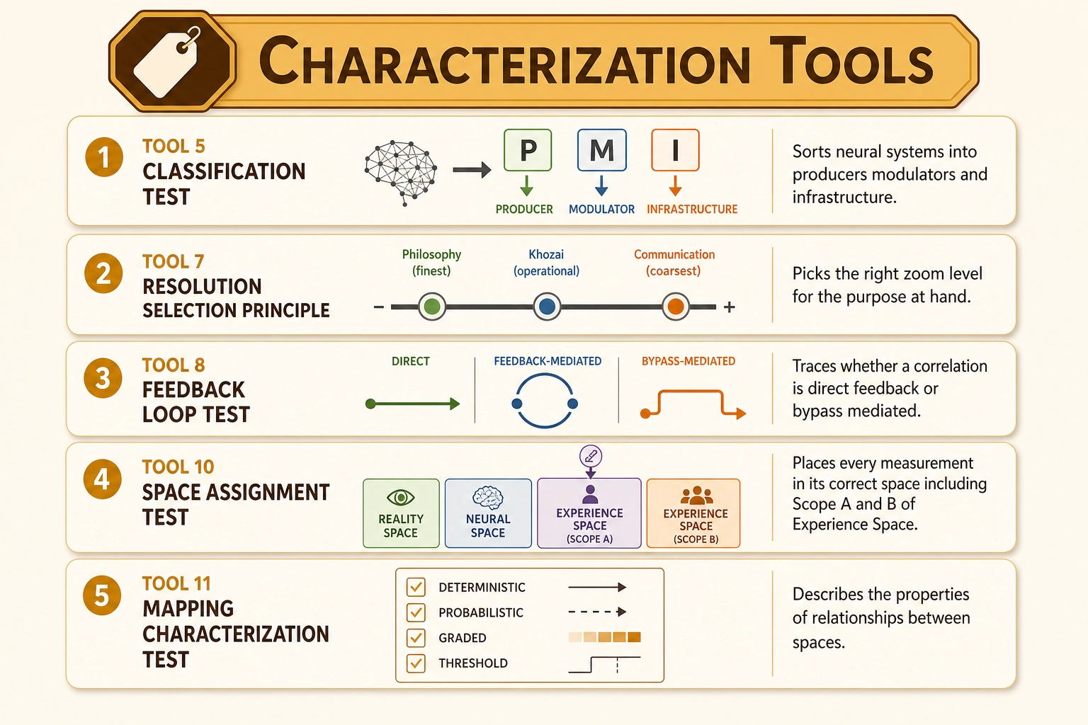
5.3. Validation Tools
These three tools ground-truth the framework against evidence and internal consistency.
Tool 9 - Grounding Test. Traces any claim back to premises. For claim C, trace: C is derived from D, which is derived from E, which follows from Premise N. If any link relies on intuition, assumption, or an unstated premise, the chain is broken. The claim is either unjustified (remove it) or requires a new premise (add one, subject to Tool 12 fact-checking).
Tool 12 - Fact Check Test. Verifies empirical claims cited in the framework. Five sub-tests: (12a) Source exists - real publication, peer-reviewed, not retracted. (12b) Accuracy - the study says what we claim it says, not mischaracterized. (12c) Methodology - adequate sample size, controls, statistical analysis, meaningful effect size. (12d) Replication - replicated by independent groups; single study = suggestive, multiple replications = established, failed replications = disqualifying or noted. (12e) Current standing - not superseded or substantially revised by more recent work.
Tool 13 - Consistency Test. Checks new claims against the existing framework. Three sub-tests: (13a) Internal - does this claim contradict any previously accepted premise, definition, or derived principle? (13b) Cross-space - do the properties defined for different spaces remain compatible? (13c) Cross-tool - do the reasoning tools produce consistent results when applied to the same question from different angles?
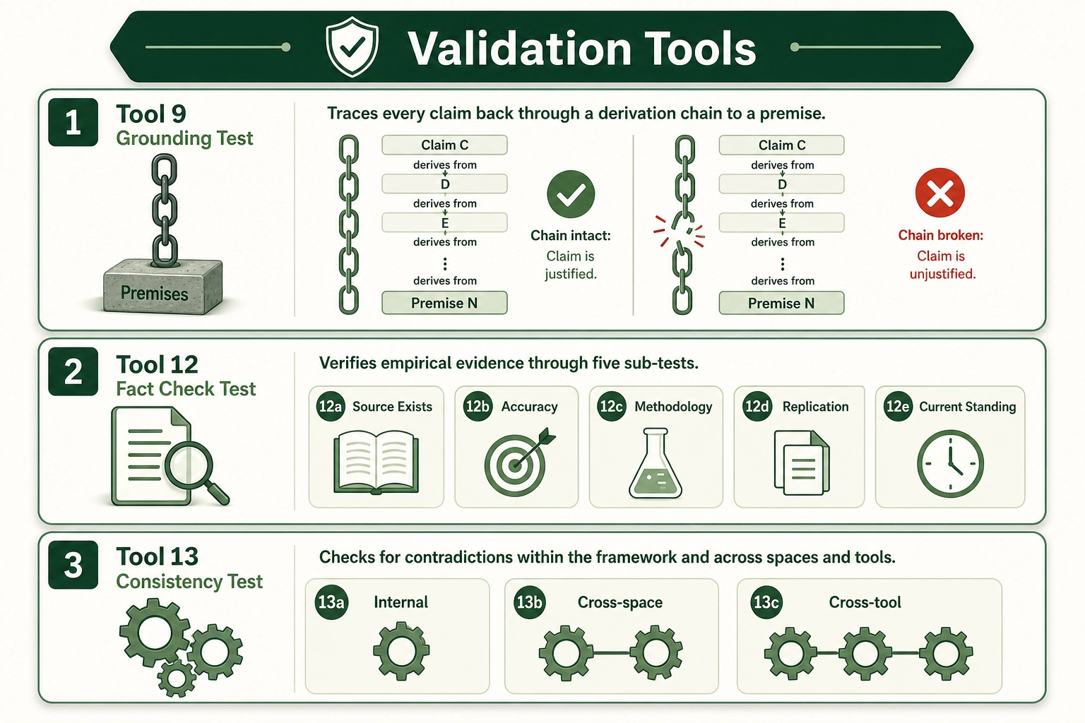
Thirteen tools cover discovery, characterization, and validation. The remaining question is: where does the framework stop? What can it claim, and what lies beyond its reach?
6. Scope Boundaries and Derived Principles
The previous five sections built the framework’s machinery: premises, spaces, mappings, vectors, and reasoning tools. This section draws the line around what that machinery can and cannot reach. It disambiguates three different uses of the word “consciousness,” states explicitly what the framework claims and does not claim, assigns an epistemological status to each space, and derives the key principles that follow from the premises through the reasoning tools. This section does not introduce new formal objects. It consolidates and constrains what the preceding sections established.
6.1. Three Senses of Consciousness
The word “consciousness” is used in at least three different ways, each with different implications for the framework:
| Sense | Definition | Scientific Status | Framework Relevance |
|---|---|---|---|
| Wakefulness | Being awake rather than asleep or in coma | Fully within science: regulated by the brainstem’s reticular activating system (RAS, the network of brainstem nuclei introduced in Section 2.3 that gates whether the cortex is online), measurable with EEG/fMRI | One dimension of Experience Space (Arousal). Well-understood. |
| Access consciousness | The ability to report on and use information consciously | Scientifically tractable: corresponds to specific neural events. The Global Neuronal Workspace theory (the neuroscientist Stanislas Dehaene et al. 2001 [11]) proposes that information becomes consciously accessible when it is broadcast across a network of interconnected cortical regions, making it available for report and flexible use | Distinguishes processing that produces Experience Space points from processing that bypasses it (Mapping 4). |
| Phenomenal experience | The subjective quality of experience: what it is LIKE | Outside current science: the hard problem (the philosopher David Chalmers 1995 [12]) | Scope B of Experience Space. The Production mapping’s mechanism. Acknowledged, not explained. |
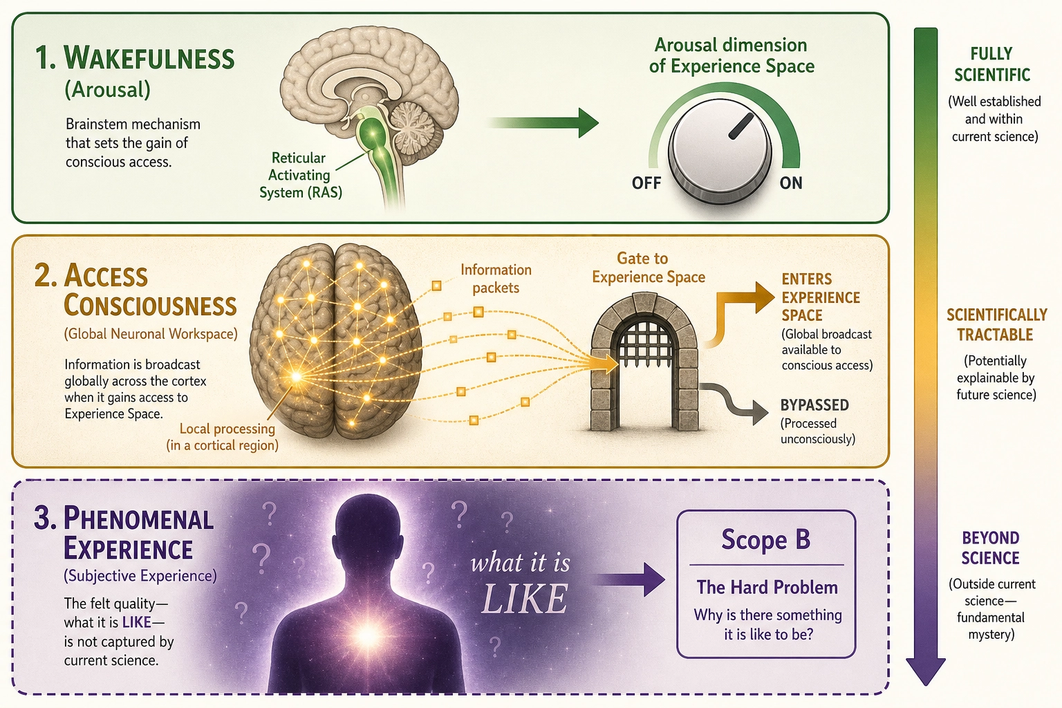
6.2. What the Framework Claims
The framework characterizes the STRUCTURE of Experience Space: its dimensions, their independence, their hierarchy, their relationship to neural hardware. This is Scope A. This is scientifically accessible through Structural Inference (Mapping 3), enabled by Premise 5. The approach is methodologically standard: characterizing properties without explaining mechanism, as Newton characterized gravity’s properties without explaining how mass curves spacetime.
6.3. What the Framework Does NOT Claim
- Does not explain WHY neural hardware produces experience (the hard problem).
- Does not claim to access the CONTENTS of experience: what red looks like, what pain feels like. Only the structure.
- Does not claim experience causes behavior: experience may be a parallel output of neural processing rather than a causal intermediary.
- Does not claim the dimension list is final: new selective eliminations could discover new dimensions.
- Does not claim one resolution is “correct”: all resolutions coexist as valid descriptions of the hierarchy.
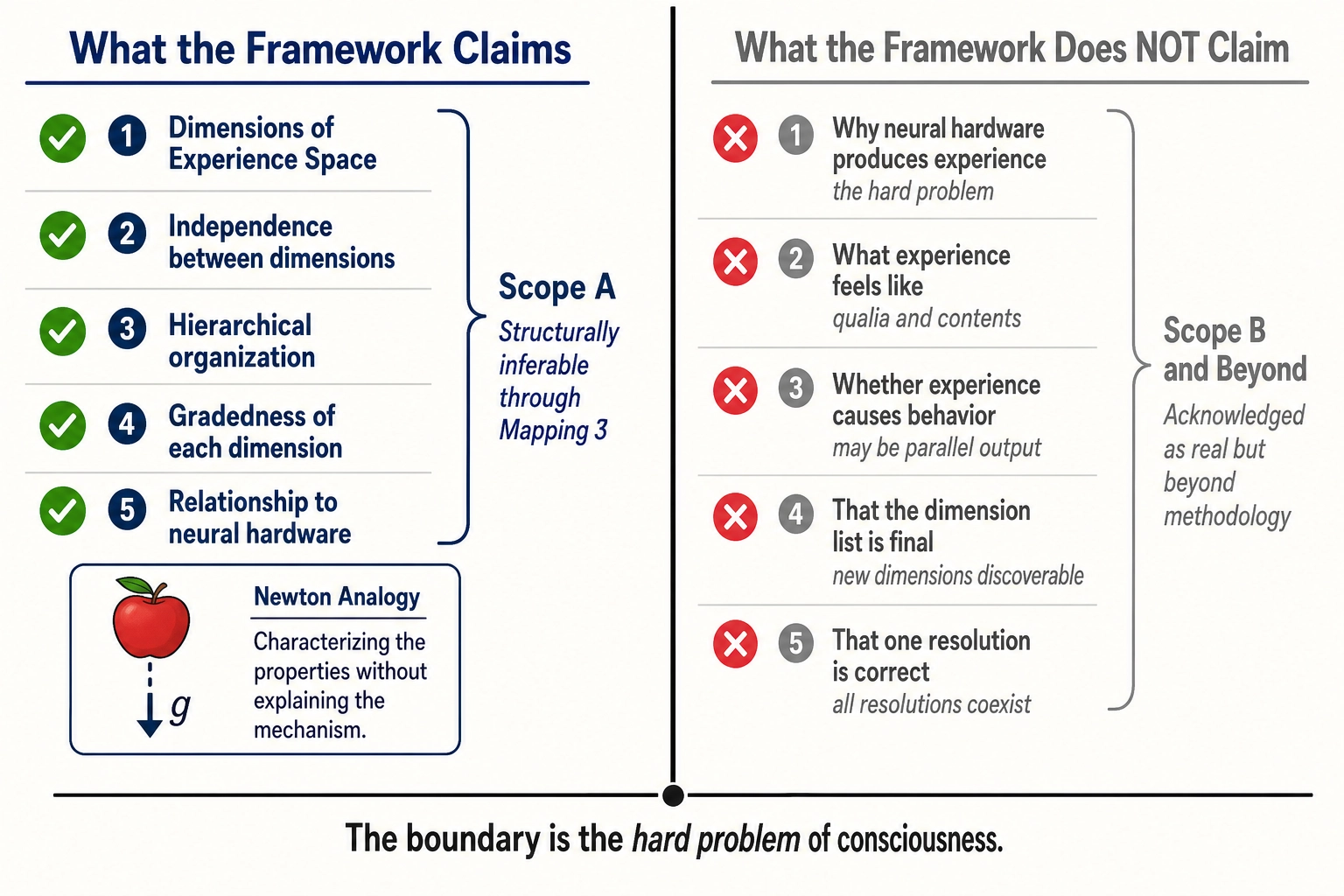
6.4. Epistemological Status of Each Space
| Space | Accessibility | Measurement |
|---|---|---|
| Physical Stimulus Space | Fully objective: any instrument can measure it | Direct, complete |
| Neural State Space | Fully objective: fMRI, EEG, electrodes can measure it | Direct but resolution-limited |
| Experience Space | Subjective: accessible only from inside. Structure (Scope A) inferable through Structural Inference (Mapping 3, enabled by Premise 5); contents (Scope B) inaccessible | Indirect only (behavioral inference, self-report) |
| Behavioral Output Space | Fully objective: observable actions, measurable metrics | Direct, complete within measured subspace |
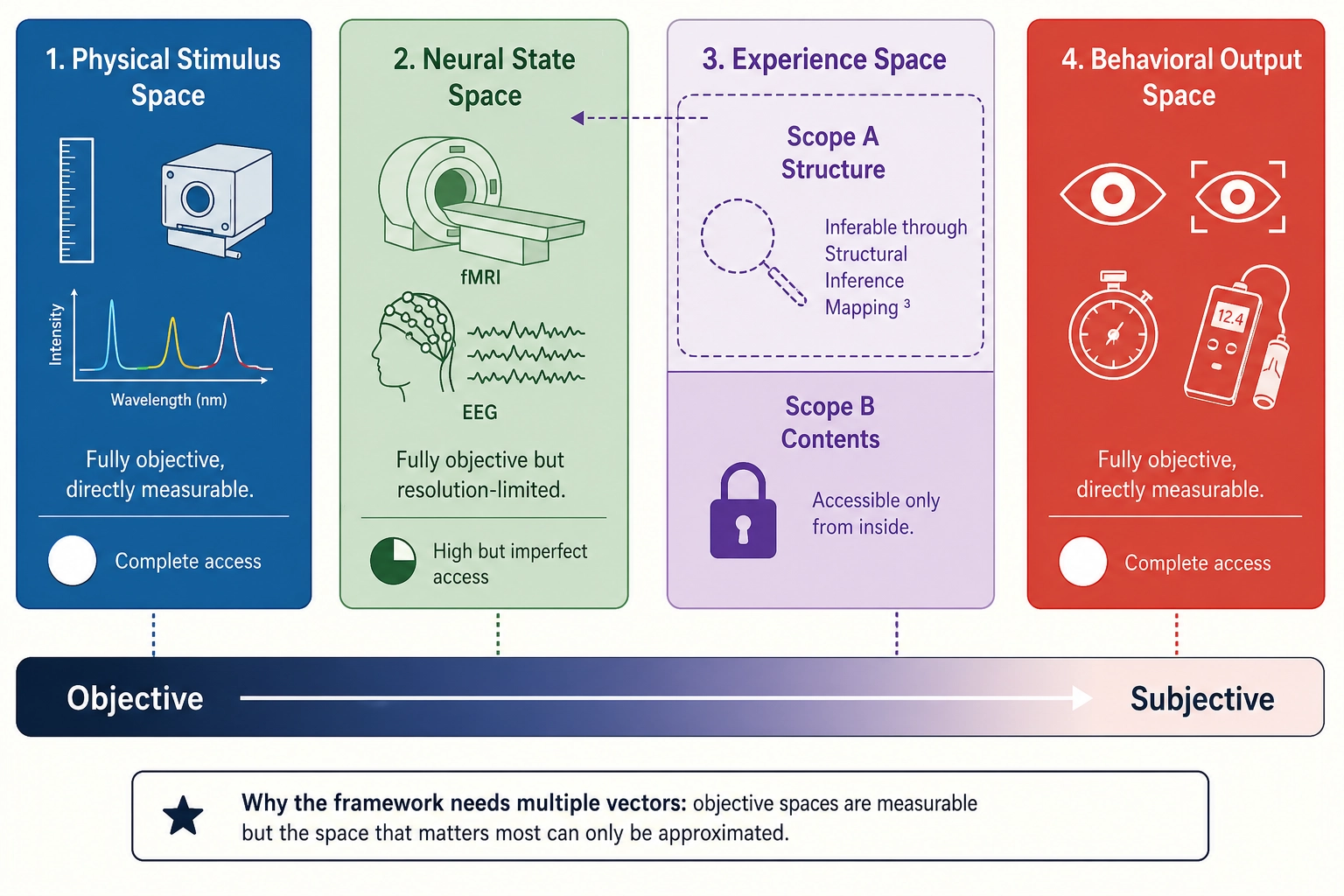
6.5. Key Derived Principles
The following principles are not premises: they are derived from the premises through the reasoning tools. Each can be traced through a derivation chain to one or more premises (Tool 9).
- Experience is decomposable. Derived from Premise 5: selective eliminations demonstrate separable components.
- Experience Space is finite-dimensional. Derived from Premises 2, 3, 4 (finite hardware) + Premise 5 (dimensions map to hardware).
- Experience Space is hierarchical. Derived from nested selective eliminations via Tool 4: destroying V1 eliminates all vision; destroying V4 eliminates only color.
- Dimensionality is resolution-dependent. Derived from the hierarchical structure: coarser resolutions are projections of finer ones. All resolutions are valid simultaneously. Premise 5 alone does not determine granularity. An additional principle (Tool 7) is needed.
- The useful resolution for Khozai is empirically determinable. Derived from the framework’s structure: the resolution at which experiential differences produce measurable behavioral differences is discoverable through the correlation engine.
- Psychological constructs are patterns, not dimensions. Derived through Tool 6 from the evidence presented in Section 2.3: constructs like anxiety decompose into configurations across existing dimensions, with no residual, and altering one component dimension transforms the experience.
- Neural State Space dimensions and Experience Space dimensions are correlated but not identical. One is objective hardware state; the other is subjective experience. Structural Inference (Mapping 3) maps architecture between them. Production (Mapping 2) maps points. They are connected but epistemologically distinct.
- The upper bound on experiential dimensions is set by hardware, not by introspection. Derived from Premises 2, 3, and 4 (finite receptor systems, finite cortical areas, finite subcortical structures) combined with Premise 5 (dimensions map to hardware). There cannot be more independent experiential dimensions than there are independent neural substrates to produce them. This means the dimension set Chapter 4 names is not merely an empirical catalog discovered by lesion studies - it is bounded above by the hardware count from Chapter 3. New dimensions can be discovered (by finding new dissociations), but the total cannot exceed the number of independently eliminable neural structures.
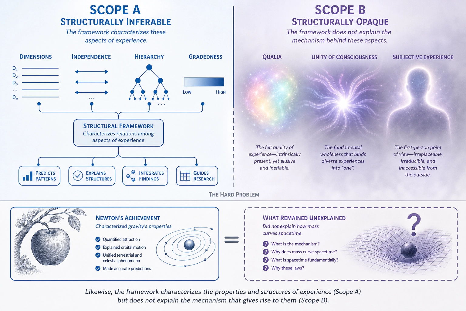
These seven principles are not additional axioms. Each traces back through a derivation chain (Tool 9) to one or more premises, with the reasoning tools providing the inferential steps. If any premise is revised, the derived principles that depend on it must be re-examined. The framework is now complete: premises, spaces, mappings, vectors, tools, scope, and the principles they jointly entail. The remaining question is what this architecture looks like when applied to real hardware.
Conclusion
This chapter defines the complete formal foundation for the Khozai project. Six premises ground everything in empirically verified facts about the brain. Four spaces define the domains of operation: physical stimulus, neural state, experience, and behavioral output. Five mappings describe how information flows between spaces, including the critical distinction between Production (point-to-point, mechanism unknown) and Structural Inference (architecture-to-architecture, the mapping the framework actually uses). The vector architecture defines what Khozai computes in each space: physics-only measurements (V0/V1/V2), cognitive approximations (Vc), cortical activation approximations (Vn), experience approximations derived from psychology (Ve), and behavioral outcomes (Vp). Thirteen reasoning tools, organized into discovery, characterization, and validation groups, provide formal operations for every type of analysis the framework requires. And explicit scope boundaries acknowledge what the framework cannot address: most importantly, the hard problem of consciousness.
Every claim in subsequent chapters traces back to the structures defined here. If a claim cannot be grounded through Tool 9, it is either unjustified or requires expanding this foundation. The framework is designed to be self-correcting: Tool 12 validates the evidence, Tool 13 catches contradictions, and the entire structure can be extended through new premises when the grounding test reveals gaps.
Chapter 3 describes the physical hardware in detail: the brain’s architecture that these premises, spaces, and mappings are about. Where this chapter defined WHAT the brain’s structures are (Premises 2-4), Chapter 3 shows HOW they operate - the thirteen properties of the brain that determine what Khozai can and cannot infer about a viewer’s response.
Bibliography
[1] Purves, D. et al. Neuroscience. 6th ed., Oxford University Press, 2018. [PEER-REVIEWED] - Used in: 1.2 (Premise 2, receptor systems inventory)
[2] Coste, B. et al. “Piezo1 and Piezo2 Are Essential Components of Distinct Mechanically Activated Cation Channels.” Science, 2010. [PEER-REVIEWED] - Used in: 1.2 (Premise 2, Piezo channel discovery)
[3] Brodmann, K. Vergleichende Lokalisationslehre der Grosshirnrinde, 1909. [PEER-REVIEWED] - Used in: 1.3 (Premise 3, original cortical parcellation)
[4] Glasser, M.F. et al. “A Multi-modal Parcellation of Human Cerebral Cortex.” Nature, 2016. [PEER-REVIEWED] - Used in: 1.3 (Premise 3, 360-area parcellation)
[5] Yeo, B.T.T. et al. “The Organization of the Human Cerebral Cortex Estimated by Intrinsic Functional Connectivity.” Journal of Neurophysiology, 2011. [PEER-REVIEWED] - Used in: 1.3 (Premise 3, 7- and 17-network solutions)
[6] Schaefer, A. et al. “Local-Global Parcellation of the Human Cerebral Cortex from Intrinsic Functional Connectivity MRI.” Cerebral Cortex, 2018. [PEER-REVIEWED] - Used in: 1.3 (Premise 3, ~400 parcel resolution)
[7] Scoville, W.B. & Milner, B. “Loss of Recent Memory After Bilateral Hippocampal Lesions.” Journal of Neurology, Neurosurgery, and Psychiatry, 1957. [PEER-REVIEWED] - Used in: 1.5 (Premise 5, patient HM)
[8] Berridge, K.C. & Robinson, T.E. “What Is the Role of Dopamine in Reward: Hedonic Impact, Reward Learning, or Incentive Salience?” Brain Research Reviews, 1998. [PEER-REVIEWED] - Used in: 1.5 (Premise 5, wanting/liking dissociation)
[9] Penfield, W. & Boldrey, E. “Somatic Motor and Sensory Representation in the Cerebral Cortex of Man as Studied by Electrical Stimulation.” Brain, 1937. [PEER-REVIEWED] - Used in: 1.6 (Premise 6, motor cortex mapping)
[10] Nisbett, R.E. & Wilson, T.D. “Telling More Than We Can Know: Verbal Reports on Mental Processes.” Psychological Review, 1977. [PEER-REVIEWED] - Used in: 2.4 (Space 4, self-report limitations)
[11] Dehaene, S. et al. “Cerebral Mechanisms of Word Masking and Unconscious Repetition Priming.” Nature Neuroscience, 2001. [PEER-REVIEWED] - Used in: 6.1 (access consciousness, Global Neuronal Workspace)
[12] Chalmers, D.J. “Facing Up to the Problem of Consciousness.” Journal of Consciousness Studies, 1995. [PEER-REVIEWED] - Used in: 3.2 (Mapping 2, explanatory gap), 6.1 (phenomenal consciousness, the hard problem)
[13] Kim, J. “Supervenience and Mind.” Cambridge University Press, 1993. [PEER-REVIEWED] - Used in: 3.2 (Mapping 2, nomological supervenience definition)
[14] Koch, C. et al. “Neural Correlates of Consciousness: Progress and Problems.” Nature Reviews Neuroscience, 2016. [PEER-REVIEWED] - Used in: 3.2 (Mapping 2, NCC research review supporting supervenience)
[15] Alkire, M.T., Hudetz, A.G. & Tononi, G. “Consciousness and Anesthesia.” Science, 2008. [PEER-REVIEWED] - Used in: 3.2 (Mapping 2, pharmacological manipulation of consciousness)
[16] Levine, J. “Materialism and Qualia: The Explanatory Gap.” Pacific Philosophical Quarterly, 1983. [PEER-REVIEWED] - Used in: 3.2 (Mapping 2, explanatory gap between neural and phenomenal)
[17] Bourget, D. & Chalmers, D.J. “Philosophers on Philosophy: The 2020 PhilPapers Survey.” Philosophers’ Imprint, 2023. [PEER-REVIEWED] - Used in: 3.2 (Mapping 2, philosophical consensus on physicalism)
[18] Masi, M. “An Evidence-Based Critical Review of the Mind-Brain Identity Theory.” Frontiers in Psychology, 2023. [PEER-REVIEWED] - Used in: 3.2 (Mapping 2, neuroscientific practice assumes supervenience)
[19] Crick, F. & Koch, C. “Towards a Neurobiological Theory of Consciousness.” Seminars in the Neurosciences, 2, 263-275, 1990. [PEER-REVIEWED] - Used in: 1.1 (Premise 1, founding the NCC research program)
[20] Wijdicks, E.F.M. et al. “Evidence-based Guideline Update: Determining Brain Death in Adults.” Neurology, 74(23), 1911-1918, 2010. [PEER-REVIEWED] - Used in: 1.1 (Premise 1, brain death criteria - cessation of brain function eliminates experience)
[21] Mai, J.K., Majtanik, M. & Paxinos, G. Atlas of the Human Brain. 4th ed., Academic Press (Elsevier), 2016. [PEER-REVIEWED] - Used in: 1.4 (Premise 4, definitive stereotaxic atlas of subcortical structures)
[22] Hawrylycz, M.J. et al. “An Anatomically Comprehensive Atlas of the Adult Human Brain Transcriptome.” Nature, 489, 391-399, 2012. [PEER-REVIEWED] - Used in: 1.4 (Premise 4, Allen Human Brain Atlas confirming closed structural ontology)
[23] Holmes, G. “Disturbances of Vision by Cerebral Lesions.” British Journal of Ophthalmology, 2(7), 353-384, 1918. [PEER-REVIEWED] - Used in: 1.5 (Premise 5, V1 lesions produce retinotopically precise blindness, graded by lesion size)
[24] Broca, P. “Nouvelle observation d’aphémie produite par une lésion de la moitié postérieure des deuxième et troisième circonvolutions frontales.” Bulletin de la Société Anatomique, 36, 398-407, 1861. [PEER-REVIEWED] - Used in: 1.6 (Premise 6, patient Leborgne - speech production loss with preserved comprehension)
[25] Hess, W.R. Das Zwischenhirn: Syndrome, Lokalisationen, Funktionen. Basel: Schwabe, 1949. [NOBEL PRIZE IN PHYSIOLOGY OR MEDICINE, 1949] - Used in: 1.6 (Premise 6, hypothalamic stimulation producing site-specific autonomic responses)
[26] Kandel, E.R., Schwartz, J.H., Jessell, T.M., Siegelbaum, S.A. & Hudspeth, A.J. (Eds.). Principles of Neural Science. 5th ed., McGraw-Hill, 2013. [PEER-REVIEWED] - Used in: 3.1 (Mapping 1, sensory transduction converts all physical energy into a common neural code)
[27] Shallice, T. From Neuropsychology to Mental Structure. Cambridge University Press, 1988. [PEER-REVIEWED] - Used in: 3.3 (Mapping 3, formal logic of inferring mental architecture from neural dissociations)
[28] Weiskrantz, L. Blindsight: A Case Study and Implications. Oxford University Press, 1986. [PEER-REVIEWED] - Used in: 3.4 (Mapping 4, behavioral response to visual stimuli without conscious visual experience)
[29] Desimone, R. & Duncan, J. “Neural Mechanisms of Selective Visual Attention.” Annual Review of Neuroscience, 18, 193-222, 1995. [PEER-REVIEWED] - Used in: 3.5 (Mapping 5, top-down attentional modulation of early visual cortex)
[30] Pool, E., Sennwald, V., Delplanque, S., Brosch, T. & Sander, D. “Measuring Wanting and Liking from Animals to Humans: A Systematic Review.” Neuroscience and Biobehavioral Reviews, 63, 124-142, 2016. [PEER-REVIEWED] - Used in: 1.5 (Premise 5, human wanting/liking operationalization inconsistencies)
[31] Berridge, K.C. “Dissecting Components of Reward: ‘Liking’, ‘Wanting’, and Learning.” Current Opinion in Pharmacology, 9(1), 65-73, 2009. [PEER-REVIEWED] - Used in: 1.5 (Premise 5, Berridge’s acknowledgment that humans cannot reliably distinguish wanting from liking introspectively)
[32] Dronkers, N.F., Plaisant, O., Iba-Zizen, M.T. & Cabanis, E.A. “Paul Broca’s Historic Cases: High Resolution MR Imaging of the Brains of Leborgne and Lelong.” Brain, 130(5), 1432-1441, 2007. [PEER-REVIEWED] - Used in: 1.6 (Premise 6, modern re-examination showing Leborgne’s lesion extended beyond Broca’s area)
[33] Dunn, J.C. & Kirsner, K. “Discovering Functionally Independent Mental Processes: The Principle of Reversed Association.” Psychological Review, 95(1), 91-101, 1988. [PEER-REVIEWED] - Used in: 3.3 (Mapping 3, critique of dissociation logic - single systems can mimic double dissociations)
[34] Wang, C.X., Hilburn, I.A., Wu, D.-A., Mizuhara, Y., Couste, C.P., Abrahams, J.N.H., Bernstein, S.E., Matani, A., Shimojo, S. & Kirschvink, J.L. “Transduction of the Geomagnetic Field as Evidenced from Alpha-Band Activity in the Human Brain.” eNeuro, 6(2), ENEURO.0483-18.2019, 2019. [PEER-REVIEWED] - Used in: 1.2 (Premise 2, preliminary evidence for human magnetoreception - not yet independently replicated)
[35] Marr, D. Vision: A Computational Investigation into the Human Representation and Processing of Visual Information. MIT Press, 1982. [PEER-REVIEWED] - Used in: 4.3 (Vc, computational vs implementation levels of analysis for Vc and Vn)
[36] Schrimpf, M., Blank, I.A., Tuckute, G., Kauf, C., Hosseini, E.A., Kanwisher, N., Tenenbaum, J.B. & Fedorenko, E. “The Neural Architecture of Language: Integrative Modeling Converges on Predictive Processing.” PNAS, 118(45), e2105646118, 2021. [PEER-REVIEWED] - Used in: 4.4 (Vn text brain similarity, transformer models predict ~100% of explainable variance in neural language responses - now contested by Hadidi et al. 2026 [51])
[37] Huth, A.G., De Heer, W.A., Griffiths, T.L., Theunissen, F.E. & Gallant, J.L. “Natural Speech Reveals the Semantic Maps That Tile Human Cerebral Cortex.” Nature, 532(7600), 453-458, 2016. [PEER-REVIEWED] - Used in: 4.3 (Vc, distributed semantic maps across cortex during naturalistic language)
[38] Mitchell, T.M., Shinkareva, S.V., Carlson, A., Chang, K.-M., Malave, V.L., Mason, R.A. & Just, M.A. “Predicting Human Brain Activity Associated with the Meanings of Nouns.” Science, 320(5880), 1191-1195, 2008. [PEER-REVIEWED] - Used in: 4.3 (Vc, text corpus statistics predict fMRI semantic activation patterns)
[39] Hauk, O., Johnsrude, I. & Pulvermuller, F. “Somatotopic Representation of Action Words in Human Motor and Premotor Cortex.” Neuron, 41(2), 301-307, 2004. [PEER-REVIEWED] - Used in: 4.3 (Vc, reading action words activates motor cortex somatotopically - embodied semantics)
[40] Mahon, B.Z. & Caramazza, A. “A Critical Look at the Embodied Cognition Hypothesis and a New Proposal for Grounding Conceptual Content.” Journal of Physiology - Paris, 102(1-3), 59-70, 2008. [PEER-REVIEWED] - Used in: 4.3 (Vc, critique of embodied semantics - motor activation may be feedback not constitutive)
[41] Yamins, D.L.K., Hong, H., Cadieu, C.F., Solomon, E.A., Seibert, D. & DiCarlo, J.J. “Performance-optimized hierarchical models predict neural responses in higher visual cortex.” PNAS, 111(23), 8619-8624, 2014. [PEER-REVIEWED] - Used in: 4.4 (Vn image brain similarity, CNNs optimized for object recognition predict V4 and IT cortex responses in macaques)
[42] Khaligh-Razavi, S.-M. & Kriegeskorte, N. “Deep supervised, but not unsupervised, models may explain IT cortical representation.” PLoS Computational Biology, 10(11), e1003915, 2014. [PEER-REVIEWED] - Used in: 4.4 (Vn image brain similarity, deep supervised CNN best explains representational geometry of human IT cortex)
[43] Xu, Y. & Vaziri-Pashkam, M. “Limits to visual representational correspondence between convolutional neural networks and the human brain.” Nature Communications, 12, 2065, 2021. [PEER-REVIEWED] - Used in: 4.4 (Vn image brain similarity, best CNNs explain ~50-60% of explainable variance in higher visual cortex - quantifies the gap with the language case)
[44] Jain, S., Vo, V.A., Lal, S. & Huth, A.G. “Better models of human high-level visual cortex emerge from natural language supervision with a large and diverse dataset.” Nature Machine Intelligence, 5, 1415-1426, 2023. [PEER-REVIEWED] - Used in: 4.4 (Vn image brain similarity, CLIP-trained models explain up to 79% of variance in high-level visual cortex, outperforming vision-only models)
[45] Conwell, C., Prince, J.S., Kay, K.N., Alvarez, G.A. & Konkle, T. “A large-scale examination of inductive biases shaping high-level visual representation in brains and machines.” Nature Communications, 15, 8859, 2024. [PEER-REVIEWED] - Used in: 4.4 (Vn image brain similarity, training data diversity and scale, not language supervision, is the primary driver of brain predictivity across 224 models)
[46] Tang, J., Du, M., Vo, V.A., Lal, S. & Huth, A.G. “Brain encoding models based on multimodal transformers can transfer across language and vision.” NeurIPS, 2023. [PEER-REVIEWED] - Used in: 4.4 (Vn cross-modal brain similarity, multimodal encoding models transfer across modalities in semantic cortical regions)
[47] Yue, X., Ni, Y., Zhang, K., Zheng, T., Liu, R., Zhang, G., Stevens, S., Jiang, D., Ren, W., Sun, Y., Wei, C., Yu, B., Yuan, R., Sun, R., Yin, M., Zheng, B., Yang, Z., Liu, Y., Huang, W., Sun, H., Su, Y. & Chen, W. “MMMU: A Massive Multi-discipline Multimodal Understanding and Reasoning Benchmark for Expert AGI.” CVPR, 2024. [PEER-REVIEWED] - Used in: 4.3 (Vc image understanding, VLM computational-level alignment - frontier models score 82-85% vs 88.6% human expert on multimodal understanding)
[48] Jiang, D., Ku, M., Wei, Z., Yang, K., Yue, X., Chen, W. & Wenhu. “CapArena: Benchmarking and Analyzing Detailed Image Captioning in the LLM Era.” ACL Findings, 2025. [PEER-REVIEWED] - Used in: 4.3 (Vc image understanding, GPT-4o matches human annotators on detailed image captioning - first model to reach parity)
[49] Fu, C., Dai, Y., Luo, Y., Li, L., Ren, S., Zhang, R., Wang, Z., Zhou, C., Shen, Y., Zhang, M., Chen, P., Li, Y., Lin, Z., Gao, J. & Qiao, Y. “Video-MME: The First-Ever Comprehensive Evaluation Benchmark of Multi-modal LLMs in Video Analysis.” CVPR, 2025. [PEER-REVIEWED] - Used in: 4.3 (Vc video understanding, frontier VLMs score 75-85% on video understanding across durations and content types)
[50] Fu, C. et al. “Video-MME-v2: A Harder Benchmark for Evaluating Multi-modal LLMs in Video Analysis.” 2026. [PREPRINT] - Used in: 4.3 (Vc video understanding, harder evaluation shows best model at 49.4% vs human expert 90.7% - video understanding remains substantially below human under rigorous evaluation)
[51] Hadidi, N., Feghhi, E., Song, B.H., Blank, I.A. & Kao, J.C. “Spurious alignment between large language models and brains can emerge from non-robust methods and overlooked confounds.” Nature Communications, 2026. [PEER-REVIEWED] - Used in: 4.4 (Vn text brain similarity, challenges Schrimpf et al. 2021’s ~100% variance claim - confounding variables perform competitively with trained LLMs)
[52] Antonello, R. & Huth, A.G. “Predictive Coding or Just Feature Discovery? An Alternative Account of Why Language Models Fit Brain Data.” Neurobiology of Language, 5(1), 64-79, 2024. [PEER-REVIEWED] - Used in: 4.4 (Vn text brain similarity, next-word prediction is not uniquely explanatory for LLM-brain alignment - many objectives discover useful linguistic features)
[53] Gao, C., Ma, Z., Chen, J., Li, P., Huang, S. & Li, J. “Increasing alignment of large language models with language processing in the human brain.” Nature Computational Science, 2025. [PEER-REVIEWED] - Used in: 4.4 (Vn text brain similarity, confirms LLM-brain alignment increases with model capability despite methodological debates)
[54] Yang, Q., Jin, H., Tang, W., Han, Q., Liu, Z., Yuan, Y., Zhao, Z. & Liu, F. “AIR-Bench: Benchmarking Large Audio-Language Models via Generative Comprehension.” ACL, 1979-1998, 2024. [PEER-REVIEWED] - Used in: 4.3 (Vc audio understanding, first comprehensive audio-language model benchmark covering speech, environmental sounds, and music)
[55] Kell, A.J.E., Yamins, D.L.K., Shook, E.N., Norman-Haignere, S.V. & McDermott, J.H. “A Task-Optimized Neural Network Replicates Human Auditory Behavior, Predicts Brain Responses, and Reveals a Cortical Processing Hierarchy.” Neuron, 98(3), 630-644, 2018. [PEER-REVIEWED] - Used in: 4.4 (Vn audio brain similarity, audio DNN predicts auditory cortex fMRI responses better than spectrotemporal models, develops separate speech/music pathways)
[56] Millet, J., Caucheteux, C., Orhan, A.E., Boubenec, Y., Gramfort, A., Dunbar, E., Pallier, C. & King, J.-R. “Toward a Realistic Model of Speech Processing in the Brain with Self-Supervised Learning.” NeurIPS, 2022. [PEER-REVIEWED] - Used in: 4.4 (Vn audio brain similarity, Wav2Vec 2.0 functional hierarchy maps onto cortical speech hierarchy, validated on 386 participants)
[57] Tuckute, G., Feather, J., Boebinger, D. & McDermott, J.H. “Many but Not All Deep Neural Network Audio Models Capture Brain Responses and Exhibit Correspondence Between Model Stages and Brain Regions.” PLOS Biology, 21(12), 2023. [PEER-REVIEWED] - Used in: 4.4 (Vn audio brain similarity, systematic comparison of audio DNNs against auditory cortex - most outpredict spectrotemporal baselines)
[58] Millet, J., Caucheteux, C., Boubenec, Y., Gramfort, A., Dunbar, E., Pallier, C. & King, J.-R. “Speech Language Models Lack Important Brain-Relevant Semantics.” ACL, 2024. [PEER-REVIEWED] - Used in: 4.4 (Vn audio brain similarity, speech foundation models capture acoustic structure but miss brain-relevant semantic representations)
[59] Russell, J.A. “A Circumplex Model of Affect.” Journal of Personality and Social Psychology, 39(6), 1161-1178, 1980. [PEER-REVIEWED] - Used in: 4.5 (Ve, foundational two-dimensional model of affective experience: valence and arousal. Replicated across languages and cultures for 40+ years)
[60] Russell, J.A. “Core Affect and the Psychological Construction of Emotion.” Psychological Review, 110(1), 145-172, 2003. [PEER-REVIEWED] - Used in: 4.5 (Ve, defines core affect as a neurophysiological state consciously accessible as a blend of hedonic and arousal values - theoretical bridge between neural states and experiential dimensions)
[61] Fontaine, J.R.J., Scherer, K.R., Roesch, E.B. & Ellsworth, P.C. “The World of Emotions Is Not Two-Dimensional.” Psychological Science, 18(12), 1050-1057, 2007. [PEER-REVIEWED] - Used in: 4.5 (Ve, four dimensions needed: evaluation-pleasantness, potency-control, activation-arousal, unpredictability-novelty. Based on 144 emotion features across multiple languages)
[62] Scherer, K.R. & Moors, A. “The Emotion Process: Event Appraisal and Component Differentiation.” Annual Review of Psychology, 70, 719-745, 2019. [PEER-REVIEWED] - Used in: 4.5 (Ve, appraisal theory: sequential evaluations of relevance, implications, coping potential, normative significance produce distinct experiential dimensions)
[63] Cowen, A.S. & Keltner, D. “Self-Report Captures 27 Distinct Categories of Emotion Bridged by Continuous Gradients.” PNAS, 114(38), E7900-E7909, 2017. [PEER-REVIEWED] - Used in: 4.5 (Ve, 27 emotion categories from 2,185 video stimuli - shows experience has more structure than dimensional models alone capture)
[64] Barrett, L.F. “The Theory of Constructed Emotion: An Active Inference Account of Interoception and Categorization.” Social Cognitive and Affective Neuroscience, 12(1), 1-23, 2017. [PEER-REVIEWED] - Used in: 4.5 (Ve, theoretical basis for Ve = f(Vc, Vn): emotions constructed from interoceptive signals + conceptual knowledge, not triggered by stimuli)
[65] Barrett, L.F., Atzil, S., Bliss-Moreau, E., Chanes, L., Gendron, M., Hoemann, K., Westlin, C. et al. “The Theory of Constructed Emotion: More Than a Feeling.” Perspectives on Psychological Science, 20(3), 392-420, 2025. [PEER-REVIEWED] - Used in: 4.5 (Ve, updated constructionist theory: signals lack inherent emotional significance, meaning derives from relational ensembles in context)
[66] Adolphs, R. & Anderson, D.J. The Neuroscience of Emotion: A New Synthesis. Princeton University Press, 2018. [PEER-REVIEWED] - Used in: 4.5 (Ve, counter-position to pure constructionism: animal studies support evolutionarily conserved neural circuits for basic emotions)
[67] Chang, L.J., Gianaros, P.J., Manuck, S.B., Krishnan, A. & Wager, T.D. “A Sensitive and Specific Neural Signature for Picture-Induced Negative Affect.” PLoS Biology, 13(6), e1002180, 2015. [PEER-REVIEWED] - Used in: 4.5 (Ve, PINES: distributed brain pattern predicted negative affect ratings in 94% of participants, 100% forced-choice accuracy, double-dissociated from pain signature)
[68] Wager, T.D., Atlas, L.Y., Lindquist, M.A., Roy, M., Woo, C.-W. & Kross, E. “An fMRI-Based Neurologic Signature of Physical Pain.” New England Journal of Medicine, 368, 1388-1397, 2013. [PEER-REVIEWED] - Used in: 4.5 (Ve, Neurologic Pain Signature: 94%+ sensitivity/specificity for pain discrimination, established methodology for brain-to-experience mapping)
[69] Lee, S.A., Lee, J.-J., Han, J., Choi, M., Wager, T.D. & Woo, C.-W. “Brain Representations of Affective Valence and Intensity in Sustained Pleasure and Pain.” PNAS, 121(25), 2024. [PEER-REVIEWED] - Used in: 4.5 (Ve, spatially non-overlapping brain representations for valence vs intensity, shared across pleasure and pain - direct evidence experiential dimensions map to separable brain patterns)
[70] Rosenberg, M.D., Finn, E.S., Scheinost, D., Papademetris, X., Shen, X., Constable, R.T. & Chun, M.M. “A Neuromarker of Sustained Attention from Whole-Brain Functional Connectivity.” Nature Neuroscience, 19, 165-171, 2016. [PEER-REVIEWED] - Used in: 4.5 (Ve, connectome-based model predicts sustained attention from brain connectivity, generalized across 6 datasets including cross-age prediction)
[71] Barrett, L.F. & Simmons, W.K. “Interoceptive Predictions in the Brain.” Nature Reviews Neuroscience, 16, 419-429, 2015. [PEER-REVIEWED] - Used in: 4.5 (Ve, brain constructs interoceptive experience through prediction rather than bottom-up sensing - basis for arousal dimension of Ve)
[72] Joffily, M. & Coricelli, G. “Emotional Valence and the Free-Energy Principle.” PLoS Computational Biology, 9(6), e1003094, 2013. [PEER-REVIEWED] - Used in: 4.5 (Ve, defines emotional valence formally as the rate of change of free-energy over time - computational formula for mapping prediction dynamics to experiential valence)
[73] Kriegeskorte, N., Mur, M. & Bandettini, P. “Representational Similarity Analysis - Connecting the Branches of Systems Neuroscience.” Frontiers in Systems Neuroscience, 2, Article 4, 2008. [PEER-REVIEWED] - Used in: 4.4 (Vn, foundational method for comparing model and brain representations - ~3,000 citations, standard tool in computational neuroscience)
[74] Dujmovic, M., Bowers, J.S., Adolfi, F. & Malhotra, G. “Obstacles to Inferring Mechanistic Similarity Using Representational Similarity Analysis.” bioRxiv, 2022.04.05.487135, 2022. [PREPRINT] - Used in: 4.4 (Vn, demonstrates that high RSA similarity does not imply mechanistic similarity - two systems can organize information similarly for different internal reasons)
[75] Sartzetaki, C., Roig, G., Snoek, C.G.M. & Groen, I.I.A. “One Hundred Neural Networks and Brains Watching Videos: Lessons from Alignment.” ICLR, 2025. [PEER-REVIEWED] - Used in: 4.4 (Vn video brain similarity, first large-scale RSA benchmarking of 99 video and image models against fMRI during video watching - temporal modeling helps early visual cortex, task relevance helps higher cortex)
[76] Fu, M., Chen, G., Zhang, Y., Zhang, M. & Wang, Y. “Comprehensive Neural Representations of Naturalistic Stimuli through Multimodal Deep Learning.” eLife, reviewed preprint, 2025. [REVIEWED PREPRINT] - Used in: 4.4 (Vn video brain similarity, VALOR video-audio-language model outperforms unimodal and static models in RSA alignment with semantic brain regions during movie watching)
[77] Oota, S.R. et al. “Task-Conditioned Probing Reveals Brain-Alignment Patterns in Instruction-Tuned Multimodal LLMs.” arXiv, 2506.08277, 2025. [PREPRINT] - Used in: 4.4 (Vn video brain similarity, instruction-tuned VLMs outperform non-instruction-tuned and unimodal models by 15-20% in encoding model prediction of brain responses during video watching)
[78] Hendrycks, D., Burns, C., Basart, S., Zou, A., Mazeika, M., Song, D. & Steinhardt, J. “Measuring Massive Multitask Language Understanding.” ICLR, 2021. [PEER-REVIEWED] - Used in: 4.3 (Vc text evidence - 57-task benchmark across STEM, humanities, social sciences; human expert baseline ~89.8%, frontier LLMs reach ~90% as of 2024)
[79] Rein, D., Hou, B.L., Stickland, A.C., Petty, J., Pang, R.Y., Dirani, J., Michael, J. & Bowman, S.R. “GPQA: A Graduate-Level Google-Proof Q&A Benchmark.” COLM, 2024. [PEER-REVIEWED] - Used in: 4.3 (Vc text evidence - 448 graduate-level science questions; PhD domain experts score 65%, frontier LLMs score ~94% as of early 2026)
[80] Phan, L., Gatti, A., Han, Z., Li, N. et al. “Humanity’s Last Exam: A Benchmark of Expert-Level Academic Questions to Assess AI Capabilities.” Nature, 649, 1139-1146, 2026. [PEER-REVIEWED] - Used in: 4.3 (Vc text evidence - 2,500 expert-authored questions; human experts ~90%, best model ~37.5% without tools as of early 2026)
[81] Caucheteux, C. & King, J.-R. “Brains and Algorithms Partially Converge in Natural Language Processing.” Communications Biology, 5, 134, 2022. [PEER-REVIEWED] - Used in: 4.4 (Vn text brain similarity - middle layers of LLMs best predict fMRI and MEG brain recordings during natural language processing, achieving near-ceiling predictions)
[82] Kumar, S., Sedlacek, S., Lokegaonkar, V. et al. “MMAU-Pro: A Challenging and Comprehensive Benchmark for Holistic Evaluation of Audio General Intelligence.” arXiv, 2508.13992, 2025. [PREPRINT] - Used in: 4.3 (Vc audio evidence - 49-skill audio reasoning benchmark; best model Gemini 2.5 Flash at 59.2% vs human experts at 77.9%)
[83] Tang, J., LeBel, A., Jain, S. & Huth, A.G. “Semantic reconstruction of continuous language from non-invasive brain recordings.” Nature Neuroscience, 26, 858-866, 2023. [PEER-REVIEWED] - Used in: 4.5 (Ve evidence - brain activation patterns decoded into continuous semantic language, demonstrating that neural-to-experiential mapping is structured enough to be inverted)
[84] Goldstein, A., Zada, Z., Buchnik, E., Sber, M., Price, A., Aubrey, B., Nastase, S.A., Feder, A., Emanuel, D., Cohen, A., Jansen, A., Gazula, H., Choe, G., Rao, A., Kim, C., Casto, C., Flinker, A., Devore, S., Doyle, W., Dugan, P., Friedman, D., Hassidim, A., Brenner, M., Matias, Y., Norman, K.A., Devinsky, O. & Hasson, U. “Shared computational principles for language processing in humans and deep language models.” Nature Neuroscience, 25, 369-380, 2022. [PEER-REVIEWED] - Used in: 4.3 (Vc - shared computational principles between brains and LLMs; neural alignment tracks next-word prediction accuracy)