Introduction
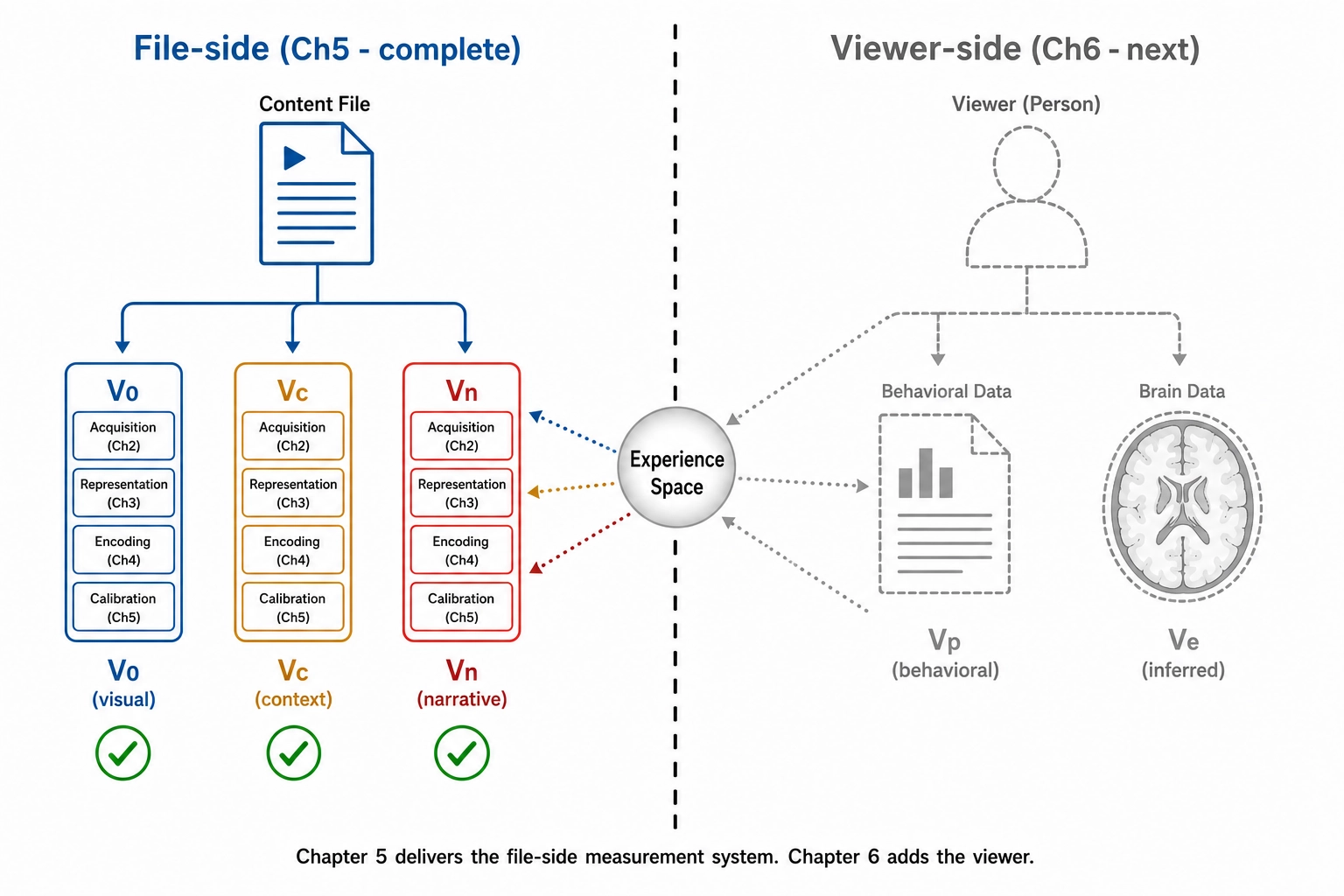
Chapter 2 set out the framework’s geography. There are four spaces: Physical Stimulus Space (the world that lands on the senses), Experience Space (what it is to be the viewer), Neural State Space (what the brain does), and Behavioral Output Space (what the viewer does next). The chapter also distinguished, inside Experience Space, between Scope A - the structure of an experience: which dimensions are involved, with what intensity, and how they relate - and Scope B - the subjective quality of any one of those dimensions, what it actually feels like from the inside. Scope A is structurally inferable from outside; Scope B is not.
Chapter 3 inventoried the hardware that produces experience: ten receptor systems, seven cortical networks, subcortical structures, and six neurochemical systems. Chapter 4 mapped the experiential dimensions onto that hardware, yielding eighteen dimensions at Resolution Level 2 with confidence tiers inherited from each dimension’s neural substrate. This chapter turns that architecture into measurement: the specific vectors Khozai computes from a content file, and the space each one lives in.
There are six vectors in scope here: V₀, V₁, V₂, Vc, Vc-temporal, and Vₙ. (Two others live outside this chapter: Vₚ lives in Behavioral Output Space and is the subject of Chapter 6; V∆, defined in Chapter 2 as the difference between a variant and a reference for any vector type, is applied in Chapter 7’s mutation engine.) Each of these six takes the same input - the content file or a parent vector’s output - and stops in a defined space.
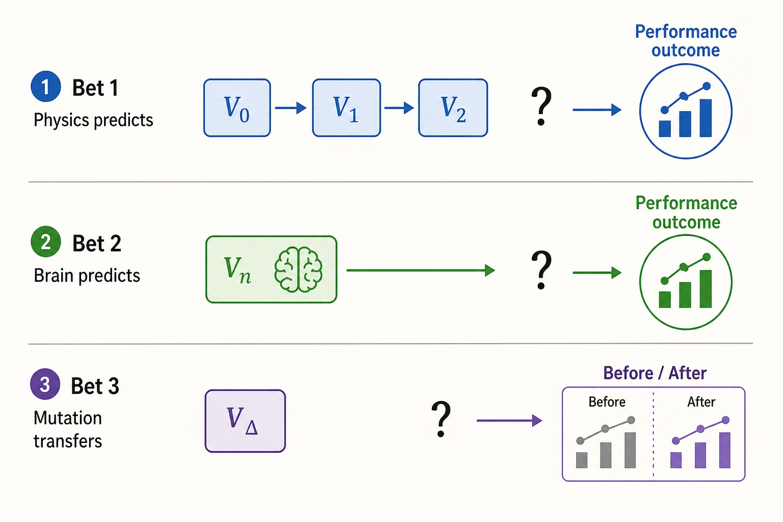
Chapter 1 framed the project around three central bets. Bet 1: physics-level content properties add predictive value beyond semantic-level properties. Bet 2: predicted brain activation from the content file alone carries enough signal to predict content performance. Bet 3: controlled single-variable mutation can reproduce and transfer success. The vectors in this chapter are the measurement instruments those bets require. V₀, V₁, and V₂ are the physics-level measurements Bet 1 depends on. Vₙ is the brain-activation prediction Bet 2 depends on. Vc provides the cognitive interpretation layer that connects physical properties to what viewers recognize. None of the bets can be tested without these vectors being specified, computed, and stored.
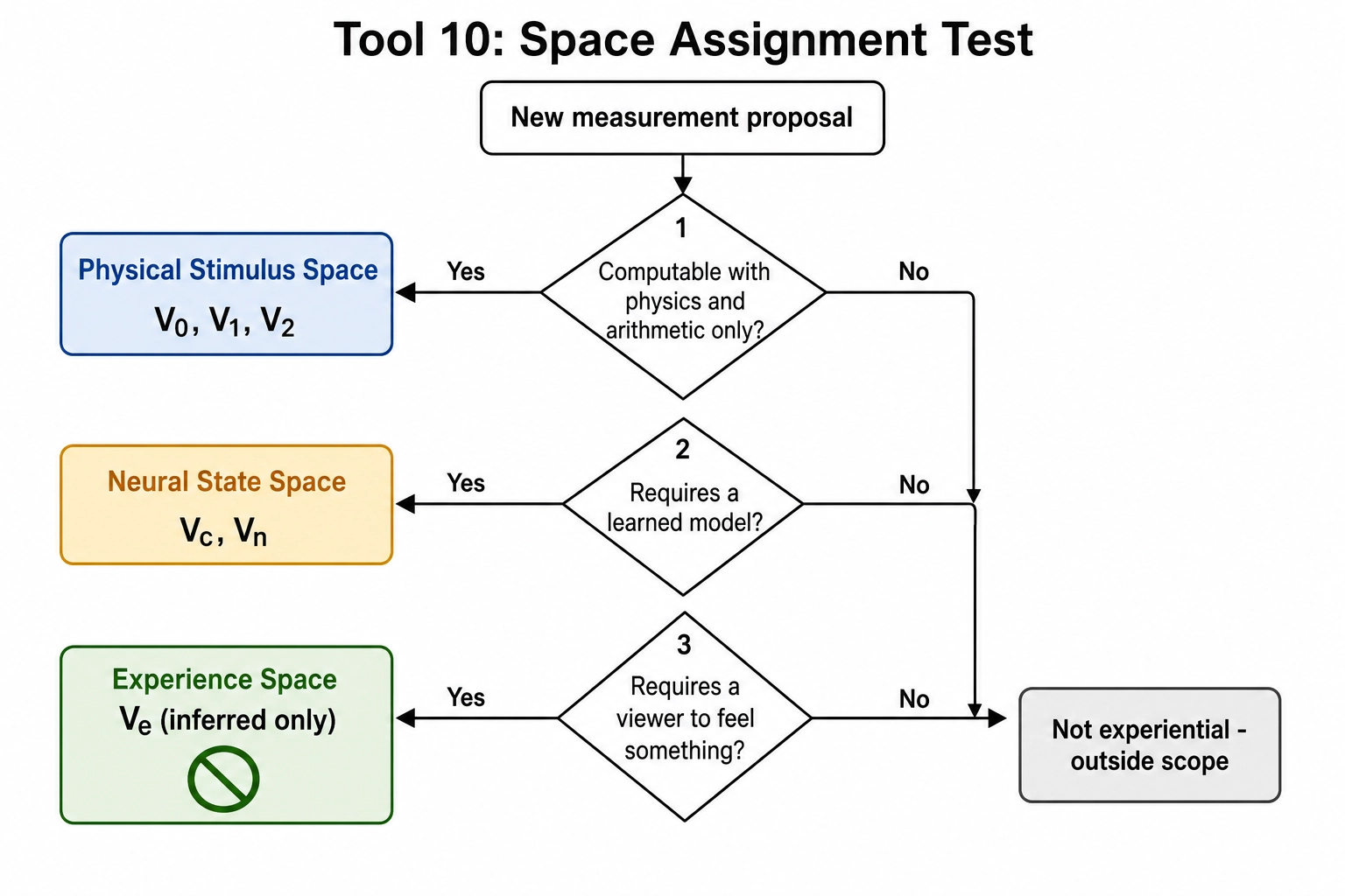
Chapter 2 named the audit that decides where a vector stops as Tool 10 (Space Assignment). The rule is operational: if a vector is computed using only physics and arithmetic on the file, it lives in Physical Stimulus Space. If its computation requires a learned model of perception, recognition, or cortical activation, it lives in Neural State Space. If it requires a viewer feeling something, it would have to live in Experience Space - and no measurement of that kind is ever made directly from the file. Every vector below is space-assigned by this rule.
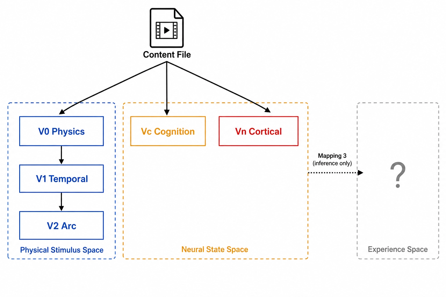
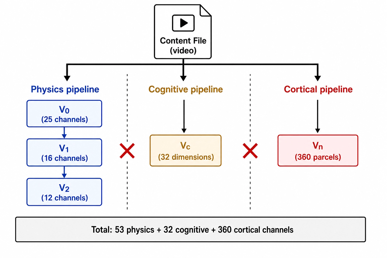
The geography of the chapter, then, is this. V₀, V₁, and V₂ live in Physical Stimulus Space. They are pixels, audio samples, and the temporal patterns of those quantities. They know nothing about people, faces, jokes, or moods. Vc and Vₙ approximate Neural State Space. Vc approximates what the brain understands (a face, a kitchen, an argument); Vₙ approximates what the brain does (which cortical regions activate, and how). Both Vc and Vₙ are model-dependent: they require systems trained on human-generated data, and both are explicitly approximations, not measurements of any individual viewer.
What is not directly computed in this chapter is Scope A of Experience Space. The structural axes of experience - sensory, affective, cognitive, motivational, bodily, and the eighteen dimensions Chapter 4 unpacked underneath them - cannot be read off the file. Chapter 2 introduced Mapping 3 - Structural Inference: the path that goes from a Neural State Space measurement, through what is known about how the cortex implements experience, to a structural inference about which experiential dimensions are engaged and how strongly. Khozai uses Mapping 3 inferentially, and validates it where it can through self-report from real viewers in Chapter 6. That validation is forward-referenced; this chapter stops at Vc and Vₙ.
| Vector | Space | Input | What it captures | Model-dependent? | Channels/dimensions |
|---|---|---|---|---|---|
| V₀ | Physical Stimulus | Content file (pixels, samples, metadata) | Instantaneous physical properties | No - deterministic physics and arithmetic | 25 channels |
| V₁ | Physical Stimulus | V₀ output | First-order temporal patterns over time windows | No - deterministic signal processing on V₀ | 16 channels |
| V₂ | Physical Stimulus | V₁ output | Second-order temporal patterns across the file | No - deterministic statistics on V₁ | 12 channels |
| Vc | Neural State (cognitive depth) | Content file (frames, audio) | What the brain understands: objects, scenes, narrative, emotion, structure | Yes - vision-language model (Gemini 2.5 Pro) | 32 dimensions |
| Vc-temporal | Neural State (cognitive depth) | Vc output (per-window values) | How cognitive dimensions change over time: arcs, peaks, trajectories | No - deterministic statistics on Vc | 24 channels |
| Vₙ | Neural State (cortical prediction) | Content file (video, audio) | What the brain does: predicted cortical activation pattern | Yes - brain encoding model (TRIBE v2) | 360 Glasser areas at 1 Hz |
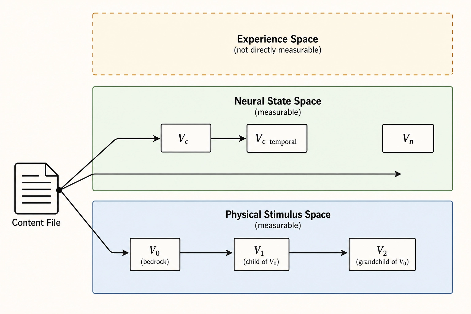
Two architectural notes set up the rest of the chapter. First, V₀, Vc, and Vₙ are siblings: each is extracted from the content file in its own pipeline, independently. V₁ and V₂ are children and grandchild of V₀; Vc-temporal is a child of Vc: V₁ is a function of V₀, V₂ is a function of V₁, Vc-temporal is a function of Vc, and none of the descendants looks at the file directly. Second, no measurement in this chapter is a measurement of any actual viewer. Vₙ in particular is a predicted pattern of cortical activation produced by a model from the file alone: no scanner, no subject, no biometric instrument. This is the property that lets the framework run at scale.
What this does NOT say. This chapter does not claim that the six vectors capture everything about a content file that matters. They capture what can be computed from the file alone, without a live viewer. It does not claim that Vc and Vₙ are measurements of experience: they are approximations of neural-state-space quantities that can be inferred to relate to experience via Mapping 3. It does not claim that subcortical predictions are as reliable as cortical ones: the confidence tiers from Chapter 3 carry through, and each vector states where its predictions are stronger and where they are weaker.
The rest of the chapter walks the six vectors in order: 1. through 3. cover the physics layers (V₀, V₁, V₂), 4. covers the cognitive layer and its temporal derivative (Vc, Vc-temporal), 5. covers the cortical approximation (Vₙ), 6. covers the architectural rationale that makes these run as parallel pipelines, and 7. covers the consistency check that makes Vc and Vₙ stronger together than either is alone.
1. V₀ - The Physics Layer
V₀ is the bedrock. Each V₀ channel is a number computed from pixels, audio samples, or container metadata using only physics and arithmetic. No perceptual model, no learned cognitive category, no human-trained transform appears anywhere in the V₀ pipeline. The V₀ specification (Phase 3, locked) commits to 25 channels in v1, partitioned into 11 pixel-domain channels, 9 audio-domain channels, and 5 container-metadata channels. The complete channel list follows, with each channel’s evidence basis for inclusion.
Pixel domain (11 channels)
Three channels anchor the pixel domain and carry the strongest evidence for predicting engagement and neural response.
v0.pixel.luminance_mean is the spatial mean of linear luminance per frame, after the standard sRGB gamma curve is removed (IEC 61966-2-1, 1999) and the Rec.709 luminance weights are applied (0.2126, 0.7152, 0.0722; ITU-R BT.709-6, 2015). The result is a physical quantity proportional to the encoded light, on a scale from 0.0 (black) to 1.0 (peak). Neither step models the human visual system. Luminance mean is a standard V1 encoding baseline (Kay et al., 2008 [7]) and a top predictor of aesthetic rating (Datta et al., 2006 [8]).
v0.pixel.frame_difference is the mean absolute pixel-by-pixel difference between consecutive frames’ linear luminance, on a [0.0, 1.0] scale. A still frame followed by an identical still frame has frame-difference 0.0; a hard cut from a black scene to a bright scene has frame-difference close to 1.0. Saying what counts as a cut is a calibration question (the threshold value lives in Chapter 10’s calibration governance). Saying what the pixel-difference number is is V₀: subtract, take absolute values, average. Pure arithmetic. Frame difference is the motion energy baseline used in every fMRI encoding model (Nishimoto et al., 2011 [9]) and predicts inter-subject neural correlation during movie viewing (Hasson et al., 2008 [10]).
v0.pixel.color_saturation_mean is the spatial mean of saturation in HSL space per frame, on a [0.0, 1.0] scale. HSL is a coordinate transform of RGB (not a perceptual model), and saturation measures color vividness. The marketing researcher Chengqi Li and colleagues (2023 [11]) showed that color complexity increases social media engagement by approximately 30% above baseline via eye-tracking; the computer scientist Ritendra Datta and colleagues (2006 [8]) found saturation among the top predictors of aesthetic rating.
The remaining eight pixel channels are presented in the table below. Each passes Tool 10: the computation is deterministic on pixels, with no learned model at any step.
![]()
| # | Channel | Computation | Output | Evidence basis |
|---|---|---|---|---|
| 1 | v0.pixel.luminance_mean | Spatial mean of linear luminance per frame | Scalar [0, 1] | V1 encoding baseline [7]; aesthetic predictor [8] |
| 2 | v0.pixel.luminance_variance | Spatial variance of linear luminance per frame | Scalar [0, +) | Contrast proxy; V1-V4 BOLD predictor in the Portilla-Simoncelli texture model [12] |
| 3 | v0.pixel.luminance_histogram | 64-bin uniform histogram of linear luminance per frame | 64-vector | Full distributional shape; texture encoding model input [12] |
| 4 | v0.pixel.luminance_entropy | Shannon entropy of the 64-bin histogram | Scalar, bits | Spatial information measure (ITU-T P.910); scene complexity indicator |
| 5 | v0.pixel.sobel_gradient_magnitude | Mean of Sobel gradient magnitude map per frame (3x3 finite-difference filter) | Scalar [0, 1] | Edge density/sharpness; no-reference quality predictor [13] |
| 6 | v0.pixel.gradient_orientation_histogram | 8-bin histogram of Sobel gradient orientations per frame | 8-vector | Captures dominant edge directions; relates to Gabor orientation selectivity in V1-V3 [7] |
| 7 | v0.pixel.spatial_frequency_spectrum | 2D FFT power binned to 8 log-spaced spatial-frequency rings | 8-vector | Coarse-to-fine spatial structure; V1-V3 encoding [9] |
| 8 | v0.pixel.spatial_frequency_slope | OLS slope of log-power vs log-frequency (the 1/f^alpha exponent) | Scalar | Naturalness index; deviations predict quality and V1 response [14] |
| 9 | v0.pixel.frame_difference | Mean absolute pixel difference between consecutive frames | Scalar [0, 1] | Motion energy baseline [9]; inter-subject correlation predictor [10] |
| 10 | v0.pixel.color_saturation_mean | Mean saturation in HSL space per frame | Scalar [0, 1] | Aesthetic predictor [8]; engagement driver [11] |
| 11 | v0.pixel.color_hue_histogram | 12-bin histogram of hue values weighted by saturation per frame | 12-vector | Color distribution; color complexity predicts engagement [11] |
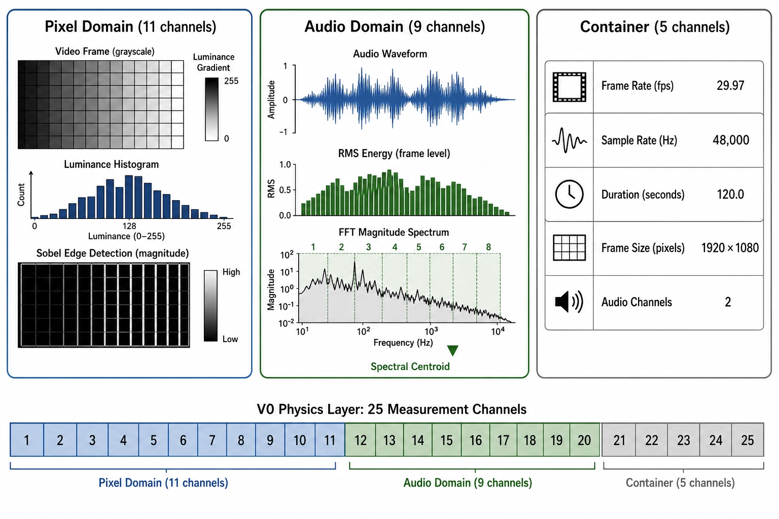
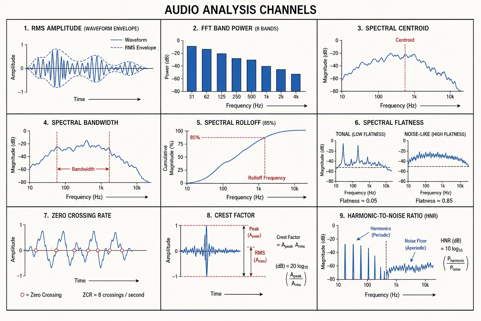
Audio domain (9 channels)
v0.audio.rms_amplitude is the root-mean-square of audio samples in Hann-windowed slices of 2048 samples (about 43 milliseconds at 48 kHz). The result is a number in [0.0, 1.0], in linear PCM units, not in decibels and not in sones. Decibels, sones, phons, LUFS: these are all perceptual scalings, calibrated to how loud a sound feels to a human, and they are explicitly excluded from V₀ on Tool 10 grounds. RMS amplitude is the strongest audio predictor of arousal (Panda et al., 2020 [15]) and a standard auditory cortex regressor (Santoro et al., 2014 [16]).
v0.audio.spectral_centroid is the frequency-weighted mean of FFT magnitudes, in hertz. It captures the “brightness” of the audio signal: high centroid means energetic, bright sound; low centroid means warm, muted sound. The spectral centroid has the strongest arousal correlation among low-level audio features (Panda et al., 2020 [15]) and is an MPEG-7 standard descriptor.
| # | Channel | Computation | Output | Evidence basis |
|---|---|---|---|---|
| 12 | v0.audio.rms_amplitude | RMS of Hann-windowed 2048-sample slices | Scalar [0, 1] PCM | Arousal predictor [15]; auditory cortex regressor [16] |
| 13 | v0.audio.fft_band_power | FFT power summed into 8 linear-frequency bands of 3000 Hz each | 8-vector | Spectral shape; foundation for V₁ spectral envelope |
| 14 | v0.audio.spectral_centroid | Frequency-weighted mean of FFT magnitudes | Scalar, Hz | Arousal/“brightness” [15]; MPEG-7 standard |
| 15 | v0.audio.spectral_bandwidth | Weighted standard deviation of frequencies around centroid | Scalar, Hz | Timbre/fullness; IRCAM core descriptor [17] |
| 16 | v0.audio.spectral_rolloff | Frequency below which 85% of spectral energy is concentrated | Scalar, Hz | Voiced/unvoiced; tension-arousal correlation [15] |
| 17 | v0.audio.spectral_flatness | Geometric mean / arithmetic mean of power spectrum (Wiener entropy) | Scalar [0, 1] | Tonality vs noise; MPEG-7 standard; voice activity detection [18] |
| 18 | v0.audio.zero_crossing_rate | Sign changes per sample per frame | Scalar, rate | Noisiness indicator; speech/music discrimination |
| 19 | v0.audio.crest_factor | Peak amplitude / RMS per window | Scalar, ratio | Dynamic compression level; AES2-2012 standard |
| 20 | v0.audio.harmonic_to_noise_ratio | Periodic energy / aperiodic energy via autocorrelation | Scalar, dB | Voice quality [19]; F0 strength; auditory cortex predictor [20] |
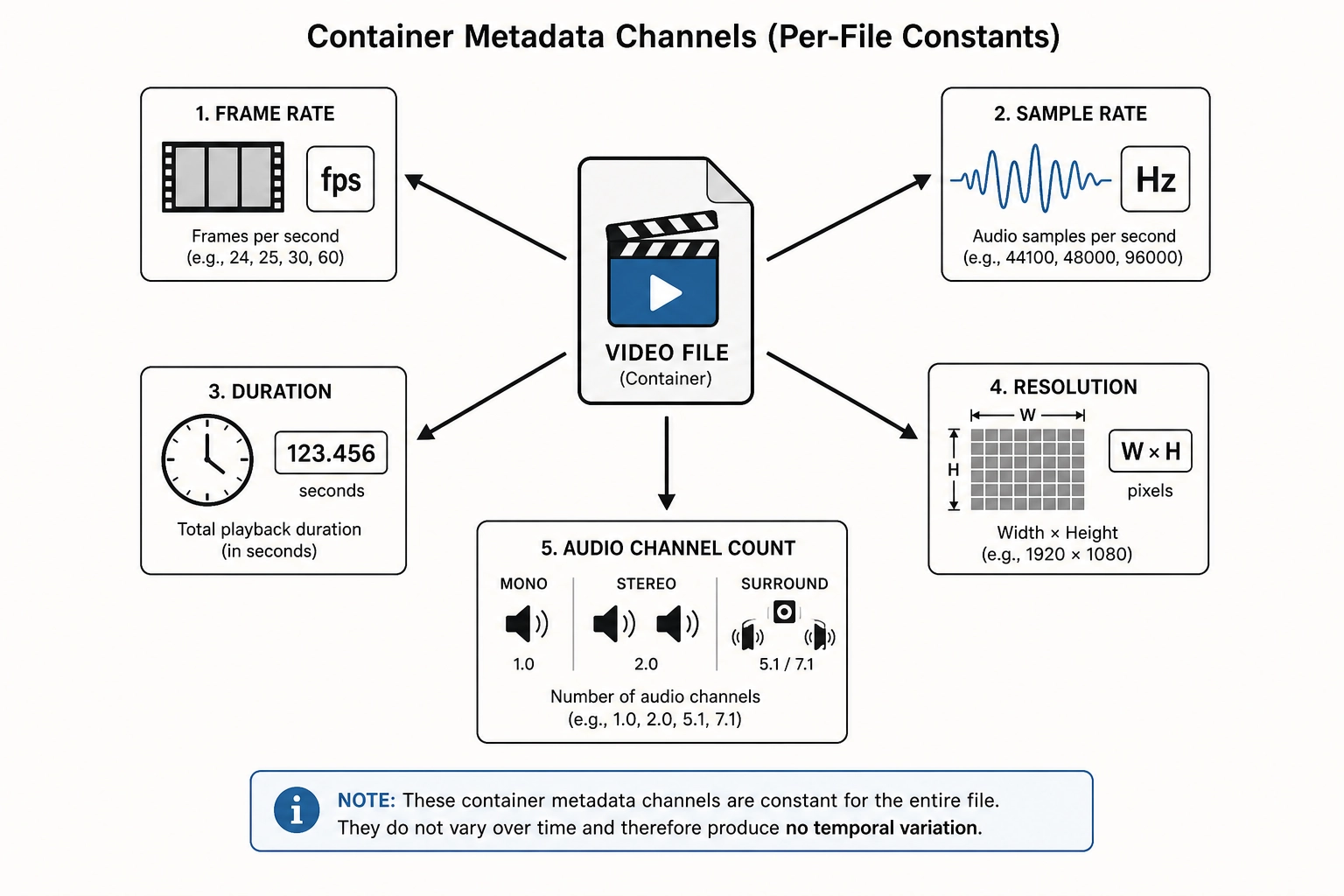
Container metadata (5 channels)
Container channels are constant per file: they carry no temporal variation and produce no V₁ signal. Their role is to provide the scaling factors and technical context without which the pixel and audio channels cannot be interpreted.
| # | Channel | Computation | Output | Role |
|---|---|---|---|---|
| 21 | v0.container.frame_rate | From container header | fps | Determines temporal resolution of all pixel channels |
| 22 | v0.container.sample_rate | From container header | Hz | Determines Nyquist limit for all audio channels |
| 23 | v0.container.duration | From container header | seconds | File-level scaling factor for V₁/V₂ windows |
| 24 | v0.container.resolution | Width x height from container header | pixels | Spatial resolution; determines pixel channel precision |
| 25 | v0.container.audio_channel_count | From container header | integer | Mono/stereo/surround; affects RMS and spectral computations |
What V₀ is not
What V₀ deliberately excludes is worth stating, because the rule it expresses is doing real work. V₀ does not contain CIELAB lightness, CIEDE2000 color distance, sones, phons, LUFS, FACS Action Units, mel-scale envelopes, saliency maps, beat tracking, music tempo, speech rate, or face area. Each of those quantities embeds a model of how a human perceives or recognizes something. They live in Vc, where model-dependence is acknowledged and managed; or in Vₙ, where it takes the form of a brain encoding model. They do not live in V₀, where the discipline is that any system analyzing the same file produces the same number. This is what Tool 10 audits, channel by channel.
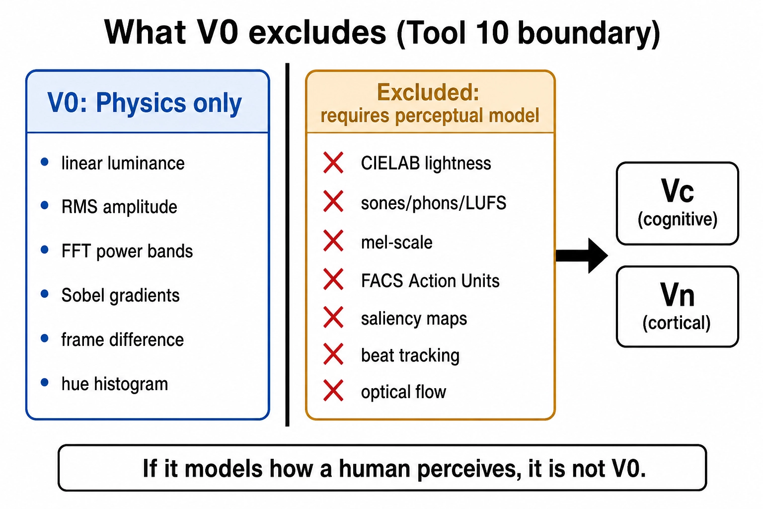
Optical flow (Lucas-Kanade, Farneback) was considered and excluded: it makes brightness-constancy and spatial-smoothness assumptions that go beyond pure arithmetic on pixels. The frame-difference channel captures the basic motion signal without those assumptions. Full Gabor filter banks (the motion energy model of the neuroscientist Shinji Nishimoto and colleagues (2011 [9])) were also excluded: they produce thousands of features, not a single channel, and belong in Vₙ’s encoding model, not in V₀’s physics layer. The spatial-frequency spectrum and gradient-orientation histogram capture the summary statistics those models operate on.
Connection to Chapter 3
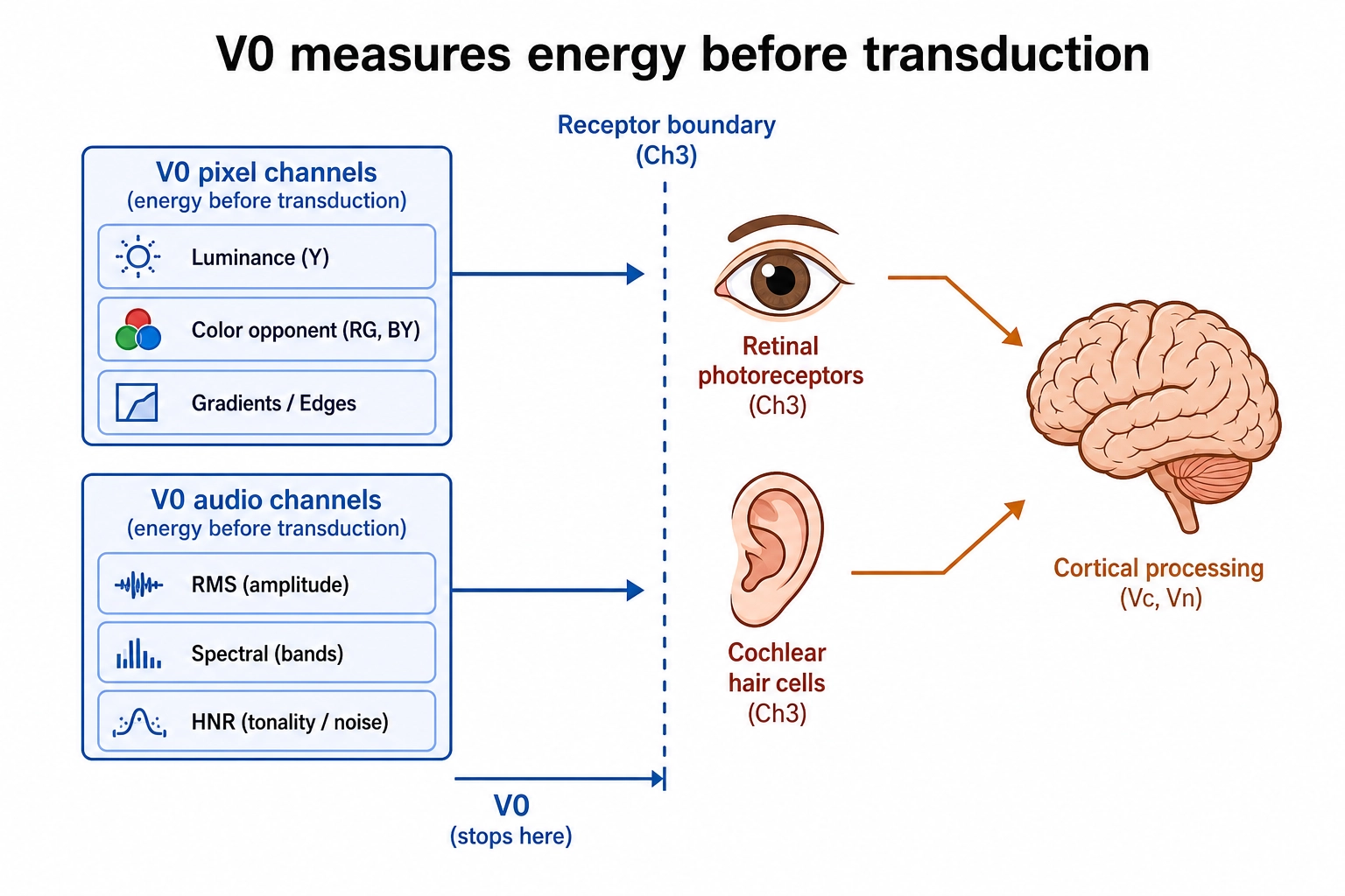
The connection to Chapter 3’s hardware inventory is direct. V₀’s pixel-domain channels measure the physical energy that Chapter 3’s visual receptor system (retinal photoreceptors, Premise 2) will transduce. V₀’s audio-domain channels measure the physical energy that Chapter 3’s auditory receptor system (cochlear hair cells) will transduce. V₀ does not model what happens after transduction: that is where the receptor system ends and the cortical processing begins, and that is where V₀ ends and Vc and Vₙ begin. The boundary is clean because biology imposes it: receptor transduction is physics; cortical processing is computation on the transduced signal.
The reason the discipline matters is structural. V₀ is the substrate against which Vc and Vₙ are checked. If V₀ smuggled in a perceptual model, the check would lose its independence: the pipeline would be comparing two model outputs, not a model output to the physics. The framework’s whole architecture rests on the V₀ side being objective in a strong sense: deterministic, reproducible, and free of human assumptions about how a stimulus feels.
Khozai implication. V₀ is the measurement layer that Bet 1 depends on. If physics-level content properties add predictive value beyond semantic-level properties (Bet 1), V₀ is where those properties live. Every V₀ channel maps to physical energy that one of Chapter 3’s receptor systems will receive, but V₀ measures the energy before transduction, not after. This is the layer where two different systems analyzing the same file must produce identical numbers: the objectivity that lets V₀ serve as the independent check on model-dependent Vc and Vₙ.
2. V₁ - First-Order Temporal Patterns
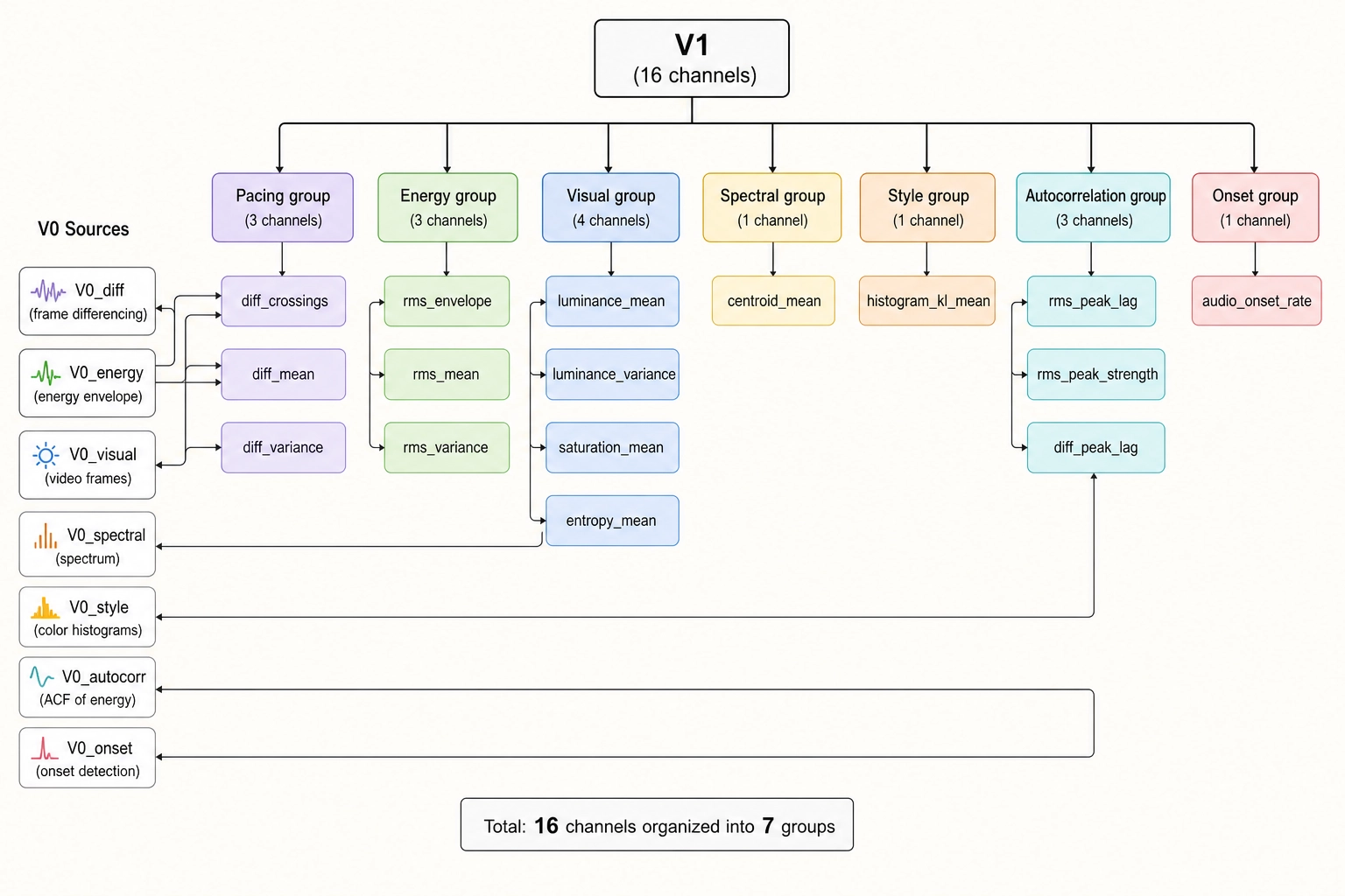
V₀ produces values at three rates: per video frame, per short audio window (about 94 times a second), and per file. V₁ takes those V₀ outputs and pools them over time. Each V₁ channel is computed from V₀ - and only from V₀ - using deterministic signal-processing or statistical operations applied over a defined window. The V₁ specification commits to 16 channels in v1, organized into pacing, energy, visual, spectral, style, autocorrelation, and onset groups.
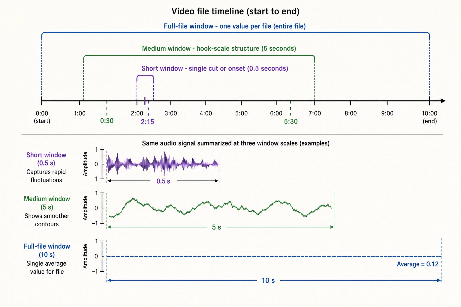
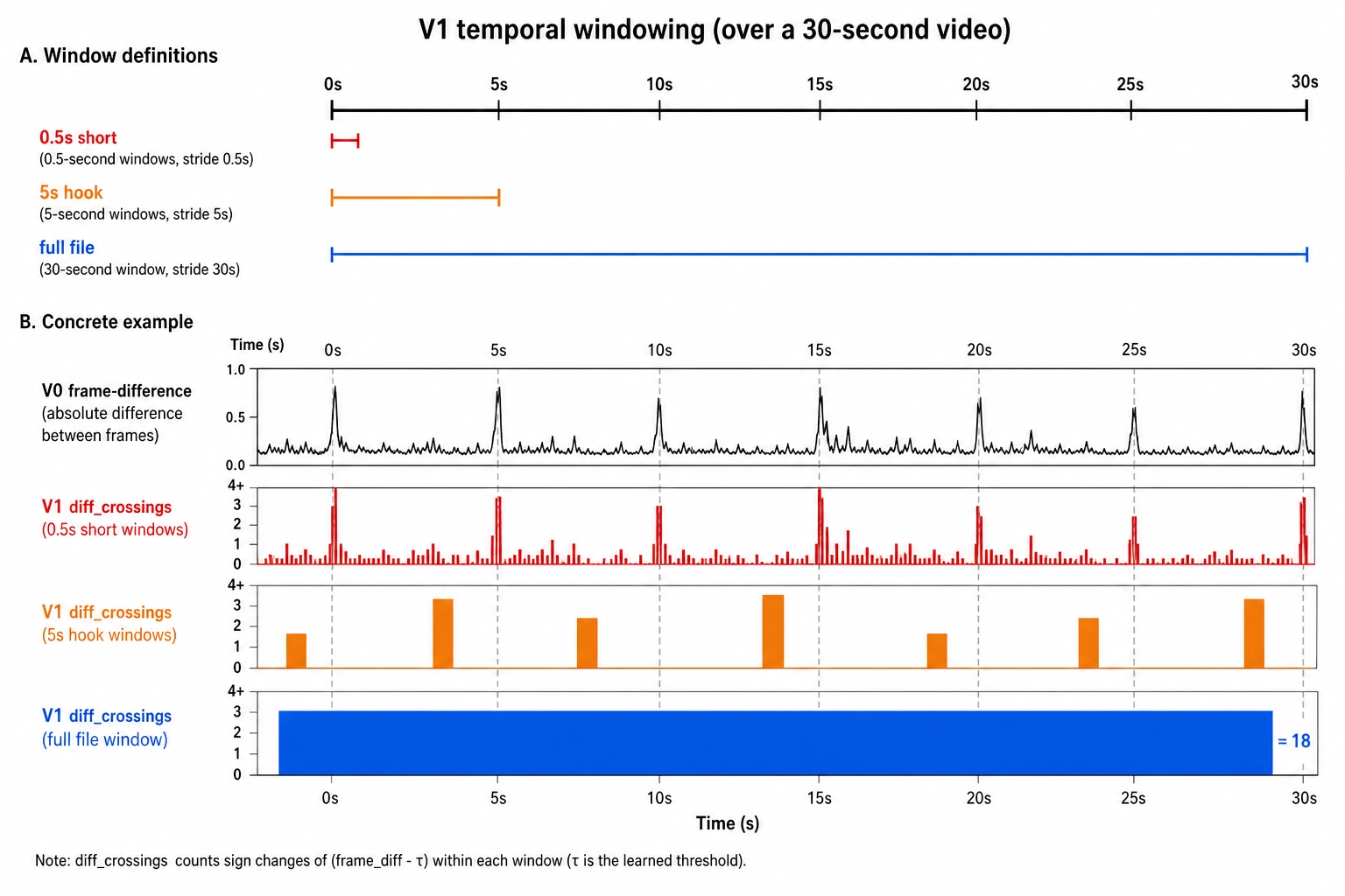
Three standard windows recur. A short window of 0.5 seconds captures rapid local pattern - a single cut, a single onset. A medium window of 5 seconds captures hook-scale structure. Research on rapid content evaluation shows the brain assesses linguistic structure in well under a second - as fast as ~130 ms for sentence-structure detection (Pylkkanen et al., 2024 [21]); the 5-second window is a conservative upper bound for hook-scale structure in short-form video. A full-file window produces one value per content file. Every V₁ channel reports at all three windows; downstream layers pick the one that fits the analysis.
Three channels deserve narrative explanation because they illustrate the V₁ design discipline.
v1.pacing.diff_crossings is the number of frames per second within a window where V₀’s frame-difference exceeds a fixed threshold. The threshold is a calibration parameter (set in Chapter 10); the operation is comparison-and-count on a physical quantity. Reading colloquially, this channel is “cuts per second,” but V₁ does not call it a cut. A learned cut-detector trained on labeled data would cross into Vc; a fixed-threshold crossing rate on V₀ pixel-difference does not. The audio researcher Juan Bello and colleagues (2005 [1]) catalog spectral-flux onset detection as a comparable family of operations on the audio side; their tutorial defines the half-wave-rectified L1 spectral flux that V₁’s audio_onset_rate channel uses verbatim, and their account confirms that this class of detector is signal processing rather than recognition.
v1.energy.rms_envelope is V₀’s RMS series resampled to a uniform 100 Hz envelope by a short moving-average low-pass and linear interpolation. The envelope is the contour of audio energy over time, a continuous trace, in linear PCM units. This is what V₂ computes its energy arc from.
v1.autocorr.rms_peak_lag is the lag at which the autocorrelation of the audio RMS envelope peaks, within a window, in seconds. If the audio has a strong rhythmic pulse at 120 beats per minute, the peak lag is 0.5 seconds. V₁ reports the lag, not “the tempo.” Calling 0.5 seconds “120 BPM” is a Vc-side interpretation; reporting 0.5 seconds is V₁.
The complete channel list follows. Note the distinction from V₀: where V₀’s luminance_variance is spatial (variation within one frame), V₁’s luminance_variance is temporal (variation across frames within a window). These capture different physical properties.
| # | Group | Channel | V₀ source | What it computes | Units |
|---|---|---|---|---|---|
| 1 | Pacing | v1.pacing.diff_crossings | frame_difference | Frames/second exceeding a fixed threshold | crossings/s |
| 2 | Pacing | v1.pacing.diff_mean | frame_difference | Average visual change rate in window | [0, 1] |
| 3 | Pacing | v1.pacing.diff_variance | frame_difference | Variability of visual change rate in window | [0, +) |
| 4 | Energy | v1.energy.rms_envelope | rms_amplitude | Audio RMS resampled to 100 Hz continuous trace | linear PCM |
| 5 | Energy | v1.energy.rms_mean | rms_amplitude | Average loudness in window | linear PCM |
| 6 | Energy | v1.energy.rms_variance | rms_amplitude | Loudness variability in window | linear PCM |
| 7 | Visual | v1.visual.luminance_mean | luminance_mean | Average brightness across frames in window (temporal) | [0, 1] |
| 8 | Visual | v1.visual.luminance_variance | luminance_mean | Brightness fluctuation across frames in window (temporal) | [0, +) |
| 9 | Visual | v1.visual.saturation_mean | color_saturation_mean | Average color vividness in window | [0, 1] |
| 10 | Visual | v1.visual.entropy_mean | luminance_entropy | Average scene complexity in window | bits |
| 11 | Spectral | v1.spectral.centroid_mean | spectral_centroid | Average audio brightness in window | Hz |
| 12 | Style | v1.style.histogram_kl_mean | luminance_histogram | Mean KL divergence between consecutive frames’ histograms | nats |
| 13 | Autocorrelation | v1.autocorr.rms_peak_lag | rms_amplitude | Dominant rhythmic period in audio | seconds |
| 14 | Autocorrelation | v1.autocorr.rms_peak_strength | rms_amplitude | Strength of dominant audio rhythm (0 = none, 1 = perfect) | [0, 1] |
| 15 | Autocorrelation | v1.autocorr.diff_peak_lag | frame_difference | Dominant visual editing rhythm period | seconds |
| 16 | Onset | v1.onset.audio_onset_rate | fft_band_power | Spectral flux peaks above threshold per second [1] | onsets/s |
Every V₁ channel declares the V₀ channel it consumes. Nothing in V₁ touches Vc or Vₙ; the sibling-and-derivation architecture from Chapter 2 4. is enforced at the channel level, not just at the framework level. The five container-metadata channels (frame_rate, sample_rate, duration, resolution, audio_channel_count) are constant per file and produce no V₁ signal; they serve as scaling factors for the channels that do vary.
Khozai implication. V₁ captures how V₀ properties change over time: editing pace, loudness contour, brightness dynamics, color vividness, visual consistency, rhythmic pulse, and audio event density. These temporal patterns are what give content its feel of speed, intensity, and momentum, but V₁ describes them in physics terms, not perceptual ones. The Tool 10 discipline is maintained one layer up: V₁ reports “0.5-second autocorrelation peak,” not “120 BPM”; it reports “diff_crossings per second,” not “cuts per second.” The perceptual label belongs in Vc. This separation matters because Bet 1 asks whether physics-level properties predict performance: if they do, V₁’s temporal patterns are a likely carrier of that signal.
3. V₂ - Second-Order Temporal Patterns
V₂ takes V₁ and asks: how does the temporal pattern itself evolve over the duration of the file? Where V₁ summarizes V₀ within a window, V₂ summarizes V₁ across windows. The V₂ specification commits to 12 channels in v1, organized into derivative, shape, and momentum groups. Operations are textbook-standard: ordinary least squares (OLS: fitting a line to data by minimizing the sum of squared residuals, the standard regression workhorse), finite differences, file-thirds comparisons, and argmax positions.
Three operation families, illustrated with examples.
Derivative (slope). v2.derivative.pacing_slope is the OLS slope of the medium-window pacing rate over the file duration - units of crossings per second per second. A positive slope means pacing accelerates over the file; a negative slope means it decelerates. v2.derivative.energy_slope does the same on the audio RMS envelope. These are not interpretations; they are linear regressions.
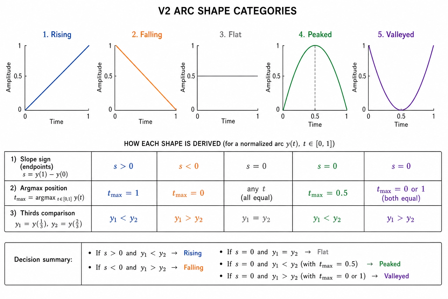
Shape (peak position + categorical label). v2.shape.energy_argmax reports the fractional position of the audio energy peak - a number in [0, 1] saying where in the file the loudest moment falls. A peak at 0.7 means the energy maxes out 70% of the way through. From these arithmetic positions, the spec defines a small set of categorical labels - rising, falling, flat, peaked, valleyed - derived by fixed thresholds applied to V₂’s own numeric outputs. A label of peaked means the argmax is in the middle third and both the first-third and last-third means are at least 30% lower than the middle-third mean. The labels are arithmetic comparisons, not learned classifiers, so they remain inside V₂’s Tool 10 envelope. The thresholds themselves (the 30%, the slope thresholds for rising versus flat) are v1 placeholders; final calibrated values come from Chapter 10.
Momentum (end vs beginning). v2.momentum.energy_change reports the difference between the last-third mean and the first-third mean of V₁’s rms_mean - how much louder (or quieter) the end of the file is compared to the beginning. v2.momentum.pacing_change does the analogous thing for pacing. v2.momentum.style_kl_drift is the OLS slope of the per-window histogram-KL divergence over time - does the visual style become more or less consistent as the file progresses.
V₂ deliberately does not assign meaning to the shape. “The energy curve rises, then peaks at 70%, then falls” is V₂. “This is a climactic structure” is Vc. The discipline is the same one V₀ and V₁ enforce on themselves: the names are arithmetic; the interpretations are explicitly a different layer.
![V2's three operation families. Derivative: OLS regression slope over file duration (positive slope means acceleration). Shape: argmax position normalized to [0,1] plus five canonical labels (rising, falling, flat, peaked, valleyed) derived from fixed thresholds. Momentum: last-third mean minus first-third mean, measuring how much a property changes from beginning to end.](/images/ch05/ch05_img26_v2_operations.webp)
The complete channel list:
| # | Group | Channel | V₁ source | What it computes | Units |
|---|---|---|---|---|---|
| 1 | Derivative | v2.derivative.pacing_slope | diff_crossings | OLS slope of pacing rate over file duration | crossings/s/s |
| 2 | Derivative | v2.derivative.energy_slope | rms_mean | OLS slope of audio energy over file duration | PCM/s |
| 3 | Derivative | v2.derivative.luminance_slope | luminance_mean | OLS slope of brightness over file duration | [0,1]/s |
| 4 | Derivative | v2.derivative.saturation_slope | saturation_mean | OLS slope of color vividness over file duration | [0,1]/s |
| 5 | Derivative | v2.derivative.complexity_slope | entropy_mean | OLS slope of scene complexity over file duration | bits/s |
| 6 | Shape | v2.shape.pacing_argmax | diff_mean | Fractional position of visual pacing peak | [0, 1] |
| 7 | Shape | v2.shape.energy_argmax | rms_mean | Fractional position of audio energy peak | [0, 1] |
| 8 | Shape | v2.shape.onset_argmax | audio_onset_rate | Fractional position of audio event density peak | [0, 1] |
| 9 | Momentum | v2.momentum.pacing_change | diff_mean | Last-third mean minus first-third mean pacing | crossings/s |
| 10 | Momentum | v2.momentum.energy_change | rms_mean | Last-third mean minus first-third mean energy | PCM |
| 11 | Momentum | v2.momentum.luminance_change | luminance_mean | Last-third mean minus first-third mean brightness | [0, 1] |
| 12 | Momentum | v2.momentum.style_kl_drift | histogram_kl_mean | OLS slope of visual consistency over file duration | nats/s |
Every V₂ channel declares the V₁ channel it consumes. V₂ never reads V₀ channels directly. The chain is V₀ → V₁ → V₂, and every step is auditable.
Khozai implication. V₂ is where the physics layers capture the arc of a content piece: does pacing accelerate toward a climax, does energy build and release, does brightness shift, does visual style stabilize or drift. These second-order patterns are the physics-level proxy for what viewers experience as narrative structure, even though V₂ never uses that word. When Chapter 7’s mutation engine changes one physical property and holds everything else constant, V₂ detects whether the change altered the arc or only the moment. The V₀ → V₁ → V₂ chain completes the physics-layer pipeline: 53 channels total (25 + 16 + 12), all deterministic, all reproducible, all auditable against the same file.
4. Vc - Cognitive Approximation
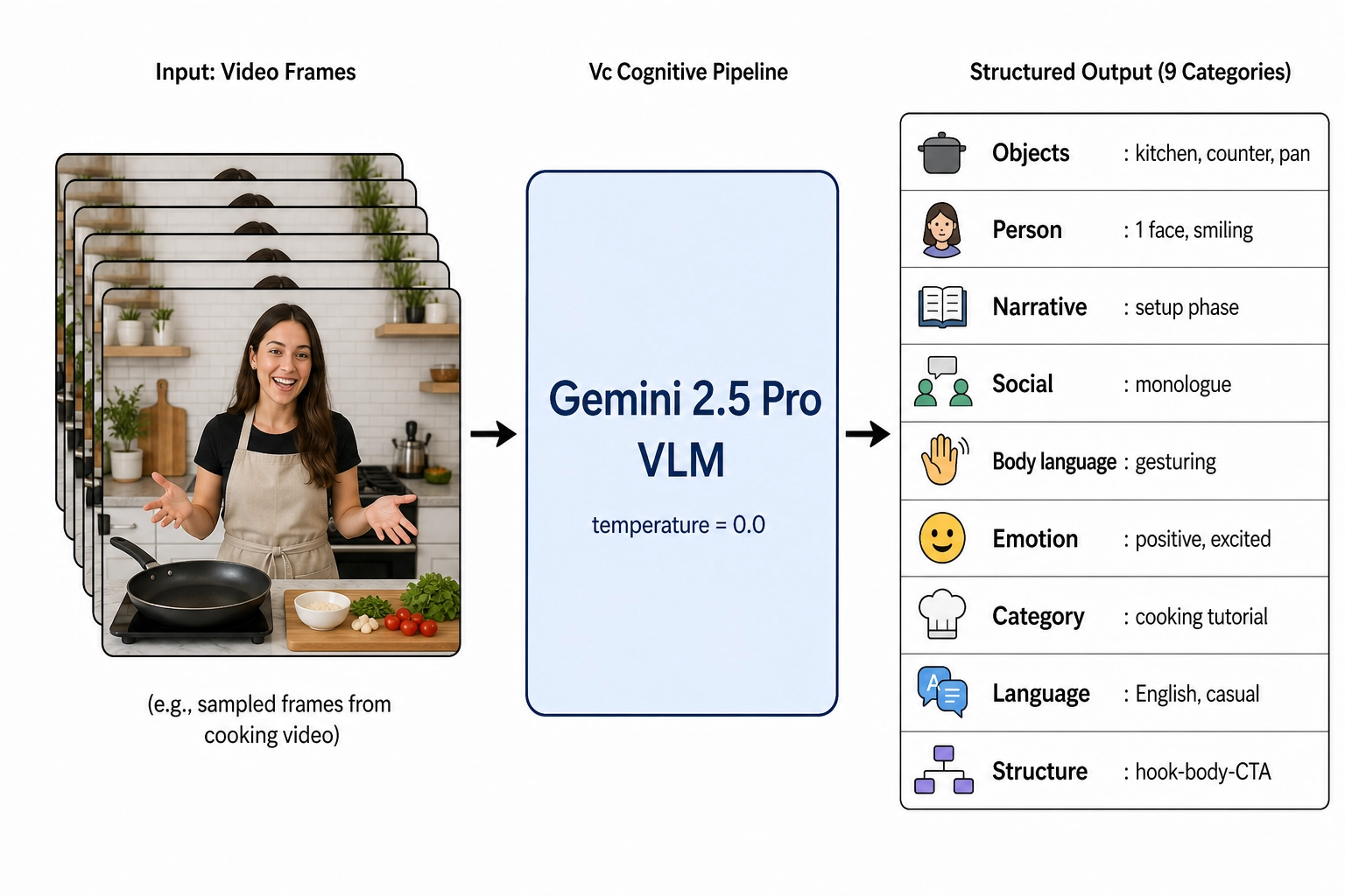
V₀ tells us that, in some frame, the linear luminance histogram has a particular shape, the spatial spectrum has a certain ring-binned profile, and the audio band powers are distributed in a certain way across 8 linear-frequency bands. V₀ does not tell us that the frame contains a woman, that she is smiling, or that the kitchen behind her has a coffee maker on the counter. A camera does not know that it sees a woman. Recognizing the woman, the smile, and the kitchen is the work of the brain’s cognitive systems, and the corresponding measurement layer is Vc.
Vc is computed by applying a vision-language model (VLM: a large language model with a visual encoder, capable of taking video frames and audio as input and producing structured text as output) directly to the content file. The model substitutes for the brain’s recognition systems. The Vc specification commits to 32 dimensions across 9 categories: object and scene identification, person attributes, narrative structure, social dynamics, body language interpretation, predicted viewer-side emotional content, content category and cultural layer, language analysis, and video structure.
Tool 10 places Vc in Neural State Space at cognitive depth. The pixels themselves are V₀; the recognition that those pixels form a face is Vc. The audio waveform is V₀; the recognition that the waveform encodes English is Vc. The Vc specification’s negative test is just as sharp: if a candidate dimension can be computed from V₀ via physics and mathematics alone, it does not belong in Vc. Cut frequency is V₁, not Vc. Narrative scene boundaries - the place where the content shifts in time, place, topic, or speaker, beyond a mere visual cut - are Vc, because identifying the narrative shift requires a model that knows what the content is about.
Some example dimensions, to make the layer concrete. vc_face_present is a per-frame boolean: does this frame contain at least one human face? vc_face_count is the integer count of distinct faces. vc_expression_primary classifies the dominant facial expression of the most prominent face from a controlled vocabulary (neutral, happy, sad, angry, surprised, fearful, disgusted, contemptuous, mixed_or_ambiguous). vc_scene_setting classifies the setting (indoor_domestic, outdoor_urban, abstract_or_graphic, etc.). vc_narrative_arc_position classifies where in a narrative arc the current window sits (setup, escalation, climax, resolution, and so on). vc_humor_structure asks whether humor is being attempted and, if so, by what mechanism (wordplay, situational, absurdist, observational, slapstick_physical, parody_or_satire, self_deprecating, dark). vc_predicted_viewer_emotion_primary is the closest Vc gets to Experience Space, and the spec is explicit that the value is a cognitive-model prediction about what the typical viewer would feel, not a measurement of what any viewer actually feels.
The model commitment is Google Gemini 2.5 Pro (released March 2025, generally available as of May 2026). The choice is documented in the Vc spec with three rationales: native multimodal video input (frames and audio as a first-class input type, without user-side frame extraction); a long context window that lets per-video analyses operate on full-length content without segmenting; and structured-output support that lets every dimension’s output conform to a JSON schema with a mandatory confidence field. The commitment is at the API tier and version-locked per snapshot; temperature is set to 0.0 (the deterministic-decoding setting where the highest-probability token is always selected) for all dimensions to reduce sampling variance. Why not alternatives? GPT-4o (OpenAI) and Claude (Anthropic) were considered. GPT-4o accepts video input but, as of May 2026, lacks native structured-output guarantees at the JSON-schema level that Vc’s pipeline requires for every dimension; a post-processing parser would introduce a failure mode the Gemini path avoids. Claude accepts image input but does not accept native video as a first-class input type, requiring user-side frame extraction that loses inter-frame and audio-visual synchronization information. Open-weight models (LLaVA-Video, InternVL) were excluded because their video context windows are shorter than commercial offerings, forcing content segmentation that introduces boundary artifacts. The pipeline is built behind a model-adapter interface so that an alternative VLM can be substituted in v2 if benchmark evidence supports it.
| Category | Representative dimensions | What it detects | Ch4 experiential dimensions engaged |
|---|---|---|---|
| Object and scene | vc_scene_setting, vc_object_count | Indoor/outdoor, objects present | Visual (RL2), Cognitive (object recognition at RL3) |
| Person attributes | vc_face_present, vc_face_count, vc_expression_primary | Faces, expressions, demographics | Visual - face recognition (RL3, FFA), Affective (valence from expression) |
| Narrative structure | vc_narrative_arc_position, vc_scene_boundary | Setup/escalation/climax/resolution, scene shifts | Cognitive (planning/sequencing at RL3), Attention (voluntary) |
| Social dynamics | vc_social_interaction_type, vc_power_dynamic | Cooperation, conflict, persuasion | Social cognition (RL2, TPJ), Self-reference (RL2, mPFC) |
| Body language | vc_gesture_type, vc_proximity | Physical stance, spatial relationships | Bodily (proprioceptive engagement via mirror system) |
| Predicted emotion | vc_predicted_viewer_emotion_primary | Predicted affective response | Affective (valence, RL2), Arousal (RL2) |
| Content category | vc_content_category, vc_cultural_register | Genre, formality, cultural context | Cognitive (semantic knowledge at RL3), Significance (RL2) |
| Language analysis | vc_language_detected, vc_speech_register | Language, tone, formality | Auditory - speech comprehension (RL3, Wernicke’s area) |
Video structure (8 dimensions)
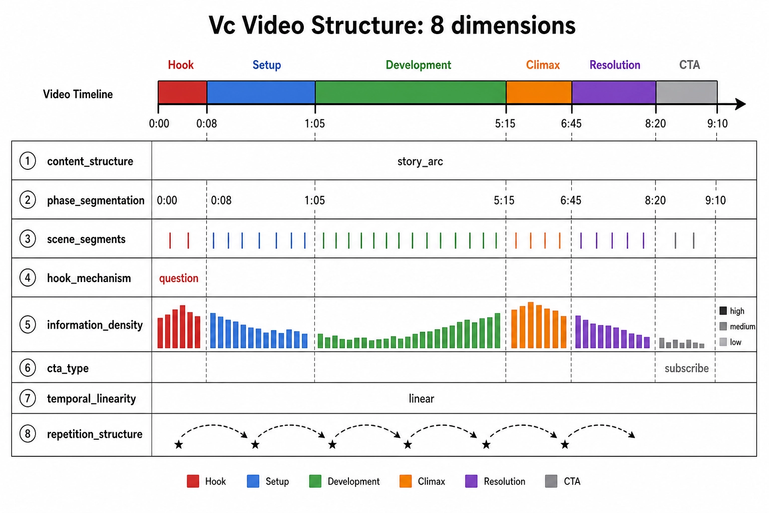
The first eight categories describe what is in each frame or window. The ninth category - video structure - describes how the content is organized over time. This distinction matters because V₀, V₁, and V₂ can detect that the pixel-difference spiked at the 3-second mark, but they cannot detect that the content shifted from a hook to a setup phase at that point. Identifying phases, scenes, and structural templates requires a model that understands what the content is about. That is Vc’s job.
The video structure category exists primarily because Chapter 7’s mutation engine needs it. If the engine wants to test “shorten the hook” or “move the climax earlier,” it must know where the hook ends and the climax begins. Per-window labels from vc_narrative_arc_position give snapshots; the structure dimensions give the full temporal map.
| Dimension | Output type | What it captures | Mutation engine use |
|---|---|---|---|
vc_content_structure | Enum: hook_body_cta, story_arc, tutorial_steps, listicle, compilation, interview, vlog, montage, reaction, before_after, other | Overall structural template of the video | Determines which mutation rules apply: a listicle can be reordered; a story arc cannot |
vc_phase_segmentation | Ordered list with timestamps: [{phase, start, end}, ...] | Full segmentation into phases (hook, setup, development, climax, resolution, CTA, outro) | Every phase-level mutation depends on this: shorten hook, extend climax, reorder phases, add/remove CTA |
vc_scene_segments | Ordered list with timestamps and attributes: [{start, end, setting, characters, tone}, ...] | Scene-level segmentation with brief description per scene | Scene-level mutations: cut a scene, swap scene order, test whether a specific scene helps or hurts retention |
vc_hook_mechanism | Enum: question, shock_surprise, tease_curiosity, visual_spectacle, direct_address, pattern_interrupt, emotional_appeal, none | How the opening grabs attention | Hook optimization is the highest-value mutation target for short-form content; knowing the mechanism enables testing alternatives |
vc_information_density | Per-window: high / medium / low | How much new information per unit time | Dense content fatigues; sparse content bores. Knowing where density spikes and drops helps the mutation engine pace edits |
vc_cta_type | Enum + timestamp: follow, like, comment, subscribe, link, purchase, none | Call-to-action presence, type, and location | CTA placement and type directly affect conversion; mutation engine can test placement, type, and phrasing |
vc_temporal_linearity | Enum: linear, flashback, parallel, circular, fragmented | Whether the timeline is straightforward or non-linear | Non-linear structures affect processing; a mutation that recuts a flashback into linear order changes the experience fundamentally |
vc_repetition_structure | Per-scene flag + pattern: recurring_motif, callback, running_gag, refrain, none | Whether and how content repeats patterns | Repetition is a known engagement driver (musical hooks, comedy callbacks); mutation engine can test adding or removing repetition |
The most critical dimension is vc_phase_segmentation. Without it, the mutation engine is blind to temporal structure. Every other structural dimension builds on or complements the phase map.
Note the cross-check with V₁ and V₂. When vc_phase_segmentation says “hook ends at 2.1 seconds,” V₁’s diff_crossings should show high visual pacing in that window. When vc_scene_segments says “scene change at 8.5 seconds,” V₀’s frame_difference should show a spike. Where the cognitive segmentation aligns with the physics signal, confidence in both rises. Where they diverge - a narrative shift with no visual cut, or a visual cut with no narrative shift - the disagreement is itself informative.
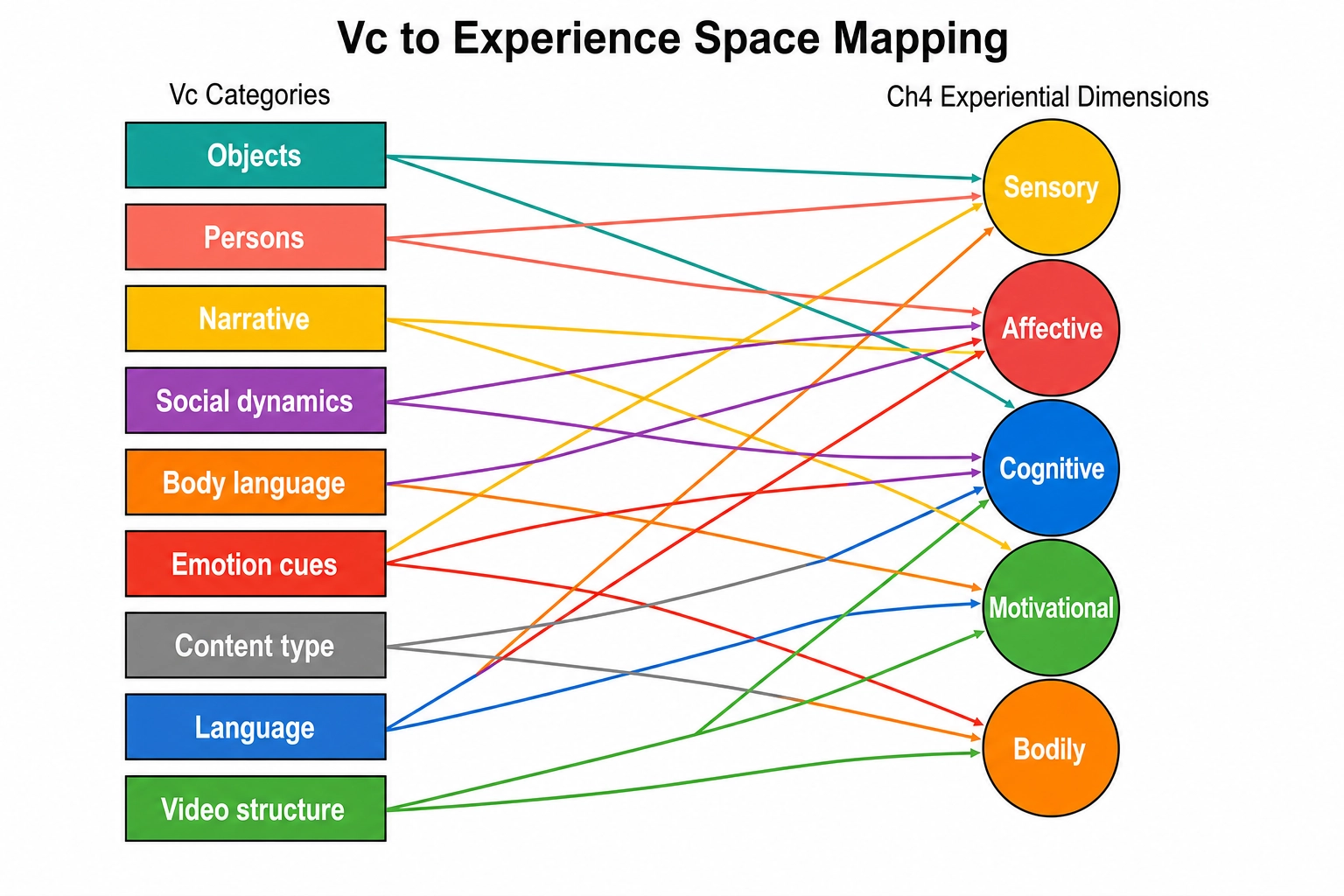
The mapping to Chapter 4’s experiential dimensions is deliberate. Vc does not measure experiential dimensions directly: it detects cognitive categories (faces, scenes, narratives, social interactions) that predict engagement of specific experiential dimensions. When Vc reports vc_face_present = true, the framework infers that the Visual - face recognition dimension (Chapter 4, RL3, FFA) is likely engaged. When Vc reports vc_social_interaction_type = conflict, the framework infers that Social cognition (Chapter 4, RL2, TPJ) and Affective (negative valence) are likely engaged. The inference is via Mapping 3 (Chapter 2): from a neural-state-space cognitive approximation, through what is known about which cortical systems implement which experiential dimensions, to a structural inference about Experience Space. Vc provides the cognitive side of that inference; Vₙ provides the cortical-activation side; Chapter 7’s consistency check compares the two.
Vc is model-dependent in a way V₀ is not. Two different VLMs may disagree on whether a face is present, on the count of people in a frame, on whether an exchange is “an argument” or “a debate,” on whether a joke landed. This is not a failure of the spec; it is a property of the layer. Cognitive categories are model-dependent in the brain too: different humans label the same scene differently. Vc’s acceptance criterion is therefore reproducibility given a fixed model, fixed prompt, fixed temperature, and fixed input frames, not bitwise objectivity. Each dimension carries a self-reported confidence score in [0, 1]. The Vc spec acknowledges that VLM self-reported confidence is known to be poorly calibrated as a standalone trust signal: the computer scientist Saurav Kadavath and colleagues (2022 [2], preprint) document the issue at length on the LLM side. Tu et al. (2024 [22]) evaluated 35 VLMs and found they are not inherently calibrated, extending the LLM finding to VLMs specifically and confirming that VLMs inherit and may amplify those limitations. For Khozai, the implication is that confidence is recorded but not trusted alone; it is one input to Chapter 8’s analysis weighting and Chapter 10’s reliability tagging, combined with internal consistency checks within Vc and the Vc-Vₙ consistency signal introduced in 7. below.
What this does NOT say. Vc does not claim to measure experience. It approximates what the brain’s cognitive systems would recognize in the content, not what a viewer would feel. It does not claim that VLM recognition matches human recognition perfectly: the acceptance criterion is reproducibility given a fixed model, not ground-truth accuracy. It does not claim that the 32 dimensions are exhaustive: they are the v1 set, subject to expansion if benchmark evidence shows missing coverage.
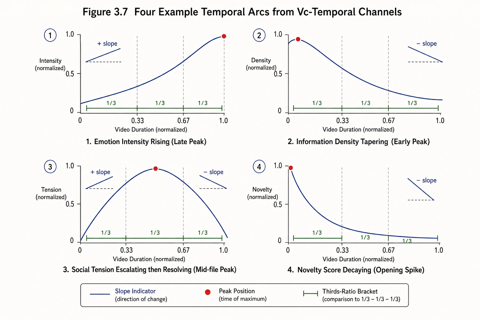
Vc-temporal: how cognitive dimensions change over time
Vc produces 32 dimensions per window. For the subset of those dimensions that are numeric and vary meaningfully across windows, the temporal pattern of that variation carries signal the per-window values alone do not. A video where vc_predicted_viewer_emotion_intensity rises steadily is structurally different from one where it peaks early and decays, even if the per-window averages are identical. The physics pipeline handles this with V₁ and V₂; the cognitive pipeline handles it with a single Vc-temporal layer computed deterministically from the per-window Vc output.
Scope. Only numeric Vc dimensions that produce a time series qualify. Categorical dimensions (vc_content_structure, vc_hook_mechanism, vc_temporal_linearity) are file-level labels with no temporal trajectory to differentiate. The qualifying dimensions are:
| Vc dimension | What its temporal pattern reveals |
|---|---|
vc_predicted_viewer_emotion_intensity | Emotional arc: rising tension, sustained peak, or early decay |
vc_information_density (coded 1/2/3) | Pacing rhythm: dense opening vs gradual build vs uniform |
vc_face_count | Social complexity trajectory: lone speaker to group to lone |
vc_object_count | Visual complexity arc: minimal to cluttered or vice versa |
vc_social_tension | Conflict arc: escalation, plateau, resolution |
vc_speech_rate | Verbal pacing: acceleration, deceleration, rhythm |
vc_body_movement_intensity | Physical energy arc: static to dynamic or peaked |
vc_novelty_score | Novelty decay: high at open, tapering as content becomes familiar |
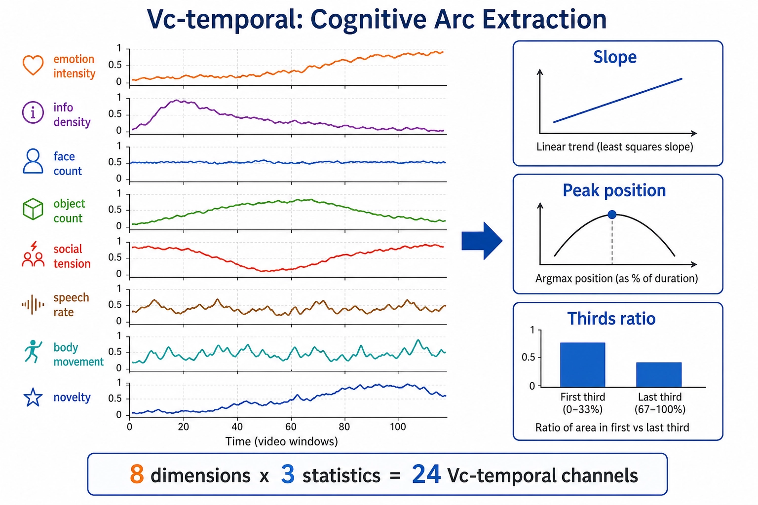
Computation. For each qualifying dimension, three temporal statistics are computed across the ordered sequence of per-window values:
| Vc-temporal channel | Computation | What it captures |
|---|---|---|
vct_slope | Linear regression slope across all windows | Overall direction: rising, falling, or flat |
vct_peak_position | Argmax normalized to [0, 1] | Where in the video the dimension peaks: early (hook), middle (climax), or late (payoff) |
vct_thirds_ratio | Mean(last third) / Mean(first third) | Whether the dimension builds or decays across the video |
![Vc-temporal computation. Eight qualifying Vc dimensions (each with a time-series sparkline) flow through three deterministic operations: slope (linear regression), peak position (argmax normalized to [0,1]), and thirds ratio (last-third mean divided by first-third mean). The result is 8 x 3 = 24 Vc-temporal channels capturing how cognitive content evolves over the video.](/images/ch05/ch05_img27_vct_computation.webp)
This yields 8 dimensions x 3 statistics = 24 Vc-temporal channels. They live in Neural State Space (same as Vc) because the underlying values are model-dependent: Vc-temporal is deterministic arithmetic on Vc output, but Vc itself requires a learned model, so the derivatives inherit that dependency. Tool 10 places them in the same space as their parent.
Why one layer, not two. The physics pipeline needs two temporal layers (V₁ for windowed statistics, V₂ for file-level arc shapes) because V₀ is a dense per-frame signal that first requires windowed summarization before arc shapes can be extracted. Vc is already at window grain: its per-window values are the equivalent of V₁. A single derivative layer (slopes, peaks, thirds-ratios) captures the arc-shape information that V₂ captures for the physics side. A second derivative would be a third derivative of the raw content, which for 8 input dimensions would produce near-zero additional variance.
Connection to the mutation engine. When the mutation engine (Chapter 7) tests “make the emotional arc peak later,” it checks vct_peak_position for vc_predicted_viewer_emotion_intensity. When it tests “increase pacing toward the end,” it checks vct_slope for vc_information_density. The Vc-temporal channels give the engine the cognitive-arc targets it needs without requiring it to recompute per-window Vc values and reason about trajectories ad hoc.
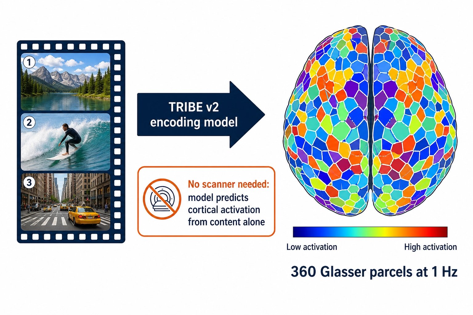
5. Vₙ - Cortical Activation Approximation
Vₙ asks a different question. Not what does the content mean? (that is Vc) but what does the brain DO when this content lands on the senses? For a given content file, Vₙ is the predicted pattern of activity across the cortical surface that an average human viewer’s brain would produce while watching that content. Vₙ is computed by a brain encoding model: a model trained on real fMRI data from real people watching naturalistic content, applied to the content file alone. There is no scanner, no live subject, no biometric equipment. The viewer is simulated, not measured.
The v1 implementation is TRIBE v2, the brain encoding model released by Meta’s FAIR team on March 26, 2026 [3] (blog post, not peer-reviewed at time of writing). While TRIBE v2 itself lacks peer review, the encoding-model class it belongs to has strong peer-reviewed grounding: the computational neuroscientist Martin Schrimpf and colleagues (2021 [23]) showed that predictive-processing language models converge with neural data across the cortical language network, and the computational neuroscientist Richard Antonello and colleagues (2023 [24]) demonstrated scaling laws for language encoding models in fMRI, establishing that model performance improves predictably with scale. According to the Algonauts 2025 organizers, TRIBE v2’s predecessor TRIBE v1 placed first among more than 260 teams [4]. Meta reports that TRIBE v2 was trained on approximately 451.6 hours of naturalistic fMRI from approximately 25 subjects across four naturalistic studies (movies, podcasts, silent videos), per the TRIBE v2 technical breakdown. It was evaluated on 1,117.7 hours from 720+ subjects in a held-out evaluation cohort. These numbers describe different things: the writing rule is to keep them separate, because conflating them inflates the apparent training scale. Based on TRIBE v2’s reported performance, the framework treats brain encoding from video as a working capability in 2026, not a speculative future tool. That is what TRIBE v2 contributes to the framework. Why not alternatives? The main competitor class is voxelwise encoding models built on smaller single-study datasets (e.g., models trained only on the Studyforrest or Courtois NeuroMod corpora). These achieve respectable within-study accuracy but have not demonstrated cross-dataset generalization at TRIBE v2’s scale; TRIBE v2’s multi-study training and its Algonauts 2025 win against 260+ teams provide the strongest available evidence of generalization. A proprietary alternative (e.g., Neuralink’s internal models) is not available for external use. If a future open-weight model demonstrates comparable cross-dataset performance, the pipeline’s model-adapter interface supports substitution.
What TRIBE v2 does not do, by itself, is prove Bet 2: that predicted cortical activation from an encoding model carries enough signal to predict performance. That is a separate empirical question, the bet the project exists to test. TRIBE v2’s existence proves the prediction is computable; whether the predicted signal is useful for the framework’s downstream purposes is what Phase 8 onward investigates. Bet 2 stays a bet here.
What Vₙ consumes, and what it does not
A point of careful framing: TRIBE v2 itself emits whole-brain predictions: about 20,484 cortical surface vertices on the fsaverage5 mesh (a standard low-resolution cortical mesh used to align results across subjects) plus about 8,802 subcortical voxels, roughly 70,000 voxels in total. Khozai consumes whole-brain predictions, both cortical and subcortical, at different confidence tiers. Cortical predictions enter at higher initial confidence (stronger fMRI SNR, better encoding-model reconstruction quality in published benchmarks). Subcortical predictions enter at lower initial confidence (weaker fMRI SNR, less validated reconstruction) but are included because the structures they represent are among the most relevant signals for content engagement.
The confidence tiers are inherited directly from Chapter 3’s hardware classification, which assigned them based on fMRI signal quality at different depths, not by judgment about which structures matter. Chapter 4 then mapped each experiential dimension to the hardware that produces it, and each dimension inherited its confidence tier. The table below shows how Vₙ’s prediction surface connects to Chapter 4’s eighteen dimensions through Chapter 3’s hardware:
| Vₙ prediction region | Ch3 hardware | Ch4 experiential dimension(s) | Confidence tier | Example Vₙ signal |
|---|---|---|---|---|
| V1, V2, V4, MT/V5, FFA, PPA, VWFA | Visual cortex (cortical surface) | Visual and 7 RL3 sub-dimensions (color, motion, faces, places, objects, words, spatial) | Higher | FFA activation predicts face-recognition engagement |
| A1, superior temporal gyrus, planum temporale | Auditory cortex (cortical surface) | Auditory and 4 RL3 sub-dimensions (speech, music, localization, environmental sounds) | Higher | Wernicke’s area activation predicts speech comprehension |
| Dorsolateral PFC, lateral parietal | Prefrontal/parietal networks | Cognitive, Attention, Agency | Higher | DLPFC activation predicts cognitive engagement |
| TPJ | Temporal-parietal junction | Social cognition | Higher | TPJ activation predicts theory-of-mind engagement |
| mPFC | Medial prefrontal cortex | Self-reference | Higher | mPFC activation predicts self-referential processing |
| Anterior insula, dACC | Salience network | Significance, Interoceptive | Higher | Anterior insula activation predicts significance |
| Amygdala | Subcortical | Fear (Affective RL3) | Lower | Amygdala prediction carries confidence differential |
| VTA, nucleus accumbens | Subcortical | Drive (wanting), Hedonic (liking) | Lower | Reward-circuit prediction inferred, not directly measured |
| Hippocampus | Deep medial temporal | Episodic memory (Cognitive RL3) | Mixed | Hippocampal prediction indirectly estimated |
| Brainstem RAS | Brainstem | Arousal | Lower | Brainstem prediction weakest, inferred from cortical correlates |
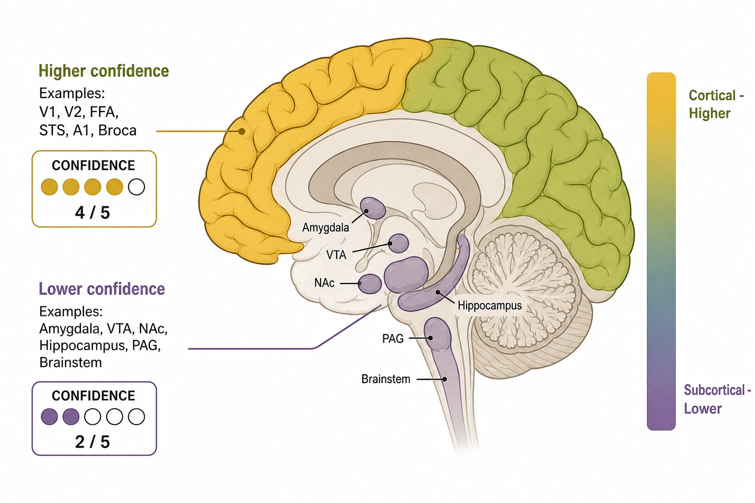
For Khozai, the implication is that confidence varies across the prediction surface, as the table above makes concrete. The confidence gap is an empirical starting point, not a permanent verdict; Chapter 10’s calibration governance tracks whether subcortical predictions earn promotion over time.
Aggregation, time, and what gets stored
The Vₙ specification applies Tool 7 (Resolution Selection): pick the coarsest aggregation at which no operationally relevant information is lost. Three candidate aggregations were considered: vertex-level (about 20,000 cortical vertices on fsaverage5), parcel-level via the Glasser 360-area multi-modal cortical parcellation, and network-level via the Yeo 7-network solution.
| Aggregation | Resolution | Verdict | Rationale |
|---|---|---|---|
| Vertex-level | ~20,000 cortical vertices | Rejected as primary (retained for diagnostics) | Too noisy for stable per-mutation comparisons, too high-dimensional to be operationally legible |
| Glasser 360 | 180 areas per hemisphere, 360 total | Locked primary representation | Fine enough to discriminate FFA from neighbors; coarse enough for legible worked examples |
| Yeo 7 | 7 cortical networks | Retained as coarse reporting tier | Right scale for summaries and Vc-Vₙ consistency checks; too coarse to distinguish within-network targets |
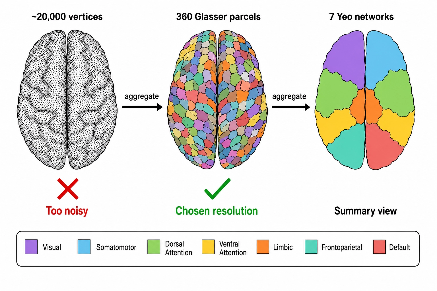
Glasser 360 is the locked primary representation. The neuroscientist Matthew Glasser and colleagues (2016 [5]) defined 180 multi-modal areas per hemisphere (360 total) using multi-modal MRI from 210 subjects in the Human Connectome Project. For Khozai, the implication is concrete: at Glasser-360 resolution, a face-area mutation produces a recognizable shift in the fusiform face area (FFA, the cortical region Chapter 3 identified as dedicated face-processing hardware and Chapter 4 mapped to the face-recognition dimension), and an audio-tempo mutation produces a recognizable shift in primary auditory cortex (A1). Both signals would be diluted at Yeo 7 and noisy at vertex level. Glasser 360 is the resolution at which the framework’s worked examples remain legible.
The Yeo 7 coarse tier is computed as a deterministic re-projection of the Glasser-tier output onto seven network masks defined by the neuroscientists Thomas Yeo and colleagues (2011 [6]), an analysis of resting-state functional connectivity in 1,000 subjects that yielded a stable 7-network and a 17-network solution. For Khozai, the implication is that the same Vₙ data can be reported at two complementary scales - fine enough to discriminate FFA from neighboring areas (Glasser 360), and coarse enough to summarize patterns across the cortex’s broad functional organization (Yeo 7) - without re-running the model.
The temporal resolution is set by the model. TRIBE v2’s native output rate is 1 Hz: one prediction per second, decimated from a 2 Hz model frequency, with a 5-second past offset compensating for the slow blood-flow change that the BOLD fMRI signal measures (BOLD: blood-oxygen-level-dependent, the standard fMRI signal that tracks blood oxygenation as an indirect proxy for neural activity). The fMRI hemodynamic response resolves at roughly 1-2 seconds; sub-second activation cannot be recovered from BOLD, and demanding a tighter time window than the model can support would manufacture precision the data does not contain. (Note: the value TR = 1.49 s appears in the TRIBE v1 Algonauts 2025 paper as the training-data repetition time and is not TRIBE v2’s output rate. Khozai consumes TRIBE v2 at native 1 Hz with no resampling.) The Vₙ schema stores a per-TR sequence at this 1 Hz cadence plus a whole-content summary frame computed by aggregating five fixed statistics - mean, peak, time-to-peak, variance, and area-under-curve - across the duration.
Average subject, license, and the three options
Two final structural limits are stated together with the confidence-tiered consumption every time Vₙ is described.
Average subject only. TRIBE v2 predicts the activation pattern an average viewer would produce, not variation across individuals, demographic strata, or psychological states. Chapter 3 stated this constraint precisely: TRIBE v2 assumes an awake, attentive viewer and cannot account for prior exposure, drowsiness, or individual differences. The neuroscientist Emily Allen and colleagues (2022 [25]) quantify the magnitude of this gap: in their massive 7T fMRI dataset, noise-ceiling SNR ranges from 0.5 to 1.25, meaning only 20-60% of variance in single-trial responses is stimulus-driven, with the remainder attributable to individual differences, internal states, and measurement noise. Persona-level evidence in Khozai accumulates on the behavioral side (Vₚ, in Chapter 6) and the self-report side, not on the Vₙ side. Vₙ remains an average-subject vector across personas.
License: CC BY-NC 4.0. TRIBE v2 is released under Creative Commons Attribution-NonCommercial 4.0 (TRIBE v2 GitHub repo LICENSE). NonCommercial as defined by the license - not primarily intended for or directed towards commercial advantage or monetary compensation - applies even to single personal users when the output is used to produce content that generates revenue. The three options for live commercial deployment are always stated together: (1) obtain a commercial license from Meta; (2) rebuild the equivalent capability on an open dataset such as CNeuroMod (~200 hours per subject, CC0 processed data, cneuromod.ca); (3) use TRIBE v2 only for non-commercial research phases. The license is a constraint that applies even if all three of Khozai’s central bets succeed. It is treated as a risk separate from the bets.
What Vₙ supports inferring, and what it does not
Khozai’s inferential claim from a Vₙ value is precise. Given a predicted activation pattern across the 360 Glasser areas at 1 Hz over the duration of a content file, Khozai can infer which aspects of the viewer’s perception and emotion are likely engaged (which Scope A dimensions of Experience Space are involved), how strongly (their relative intensity), and how independently (whether several dimensions are co-engaged or whether one dominates). It uses the rest of the framework - Mapping 3 from Chapter 2, the Scope A dimensions from Chapter 4, and the hardware-to-dimension mapping from Chapter 3 - to do this inference. The table above makes the inference path concrete: a Vₙ pattern showing elevated FFA activation is inferred, via Mapping 3, to indicate engagement of the face-recognition dimension (Chapter 4, RL3, higher confidence); a pattern showing elevated amygdala activation is inferred to indicate fear engagement (Chapter 4, RL3, lower confidence). The confidence tier travels with the inference.
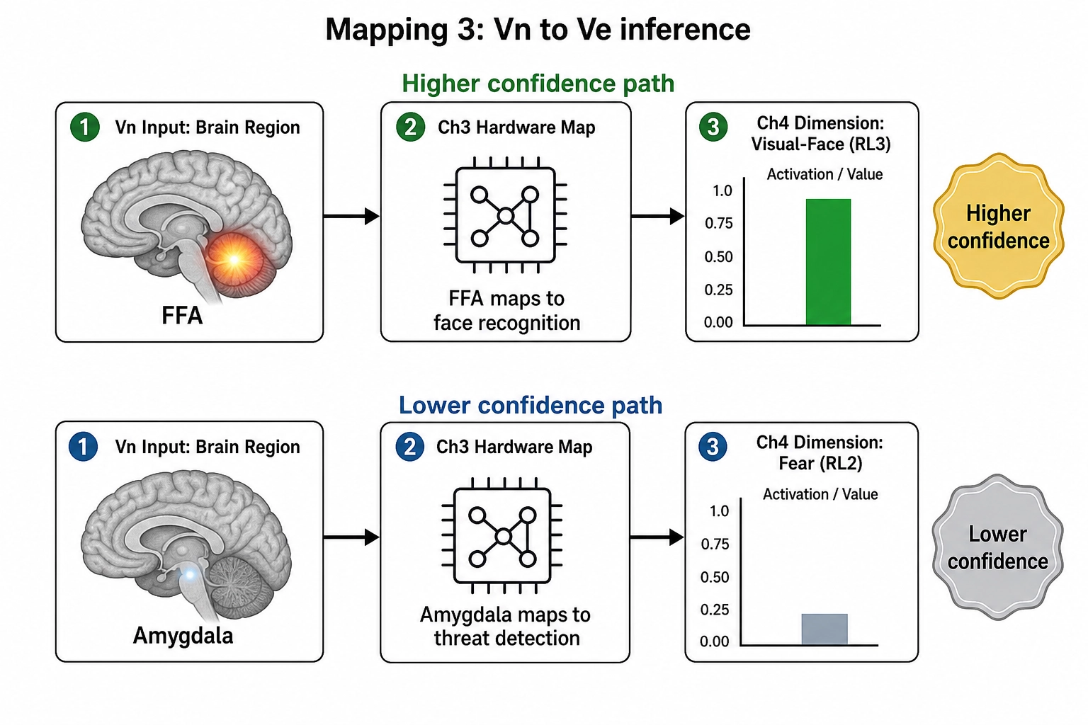
What Khozai cannot infer from Vₙ is what any of it feels like. That is Scope B of Experience Space, and it is not directly measurable from the file. The which / how-strongly / how-independently / never-what-it-feels-like discipline is the same one Chapter 2 introduced, applied to the cortical layer. Additionally, Chapter 3 established that encoding models cannot see which neurochemical caused a cortical change: Khozai sees the cortical temperature change but cannot see which dial was turned.
What this does NOT say. Vₙ does not claim to measure brain activity: it predicts what brain activity an average viewer would likely produce, using a model trained on real fMRI data. It does not claim that subcortical predictions are as reliable as cortical ones: the confidence tiers from Chapter 3 carry through explicitly. It does not claim that TRIBE v2 is the only possible implementation: the pipeline is designed to accept alternative brain encoding models if future evidence supports a switch. It does not claim that Bet 2 is proven: the bet remains open until Phase 8’s empirical tests.
6. Sibling Architecture
The introduction stated the architectural fact: V₀, Vc, and Vₙ are siblings (each processing the file independently), with V₁/V₂ descending from V₀ and Vc-temporal descending from Vc. Now that each vector has been specified, the consequences of that architecture can be stated precisely.
The reason this matters operationally: V₀ is a designed channel set, locked at 25 channels in v1. If the V₀ designers (fallibly, in v1) miss a physical property that turns out to matter, the V₀-V₁-V₂ chain loses it. Vc and Vₙ are not subject to that loss in the same way. Vc and Vₙ each process the full raw content (every pixel, every audio sample, every word) through models trained on human-generated data. If V₀ fails to enumerate some physical property the model picks up on, Vc may still recognize the cognitive correlate, and Vₙ may still predict the cortical correlate. The three pipelines have overlapping coverage of the file because they go straight to the source; they do not share a bottleneck.
This is not a claim that V₀ is replaceable. The discipline V₀ enforces (objectivity, reproducibility, no perceptual model) is exactly what Vc and Vₙ are not. V₀ is the substrate against which the model-dependent vectors are checked. V₀’s value is its incorruptibility; Vc’s and Vₙ’s value is their independent coverage of the file. The architecture uses both.
For Khozai, the implication is that the sibling architecture is the framework’s insurance against omission. If any single pipeline has a blind spot, the other two can still capture the signal from the file. This is not redundancy for its own sake: each pipeline sees the content through a fundamentally different lens (physics, cognition, cortical activation), and the disagreements between them are as informative as the agreements. Section 7 describes how those agreements and disagreements are used.
A dependency chain worth making explicit: the sibling architecture’s value rests on Tool 10 (Space Assignment) from Chapter 2. V₀’s incorruptibility - the fact that it contains no perceptual model and produces identical numbers from any system analyzing the same file - is what makes V₀ a valid independent check on the model-dependent Vc and Vₙ. That independence is what makes the Vc-Vₙ consistency signal (Section 7) trustworthy: two model-dependent vectors agreeing is informative only if neither was influenced by the other or by a shared model assumption. And the consistency signal is what makes the multi-vector architecture more than redundancy - it produces a confidence gradient that no single vector could generate alone. If Tool 10 enforcement were relaxed and a perceptual model were smuggled into V₀, V₀ would cease to be an independent check, the consistency signal would lose its epistemic foundation, and the entire confidence architecture would collapse into comparing model outputs against each other. Tool 10 is the load-bearing discipline of the architecture.
7. Vc-Vₙ Consistency as Confidence
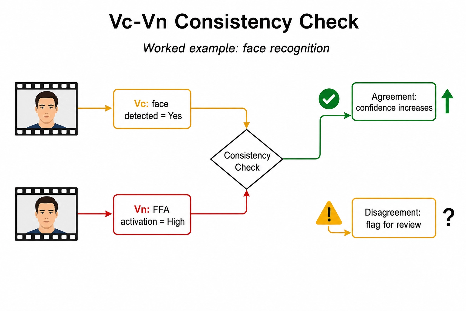
The clearest payoff of the sibling architecture is the consistency check between Vc and Vₙ. The check works because both vectors approximate aspects of the same brain from the same content file, but through independent models with independent assumptions. Where they agree, confidence rises; where they disagree, a flag is raised.
The table below shows three worked examples, each grounded in a specific Chapter 4 dimension and the Chapter 3 hardware it maps to.
| Vc signal | Expected Vₙ pattern | Ch4 dimension | Ch3 hardware | Confidence tier | Agreement meaning |
|---|---|---|---|---|---|
vc_face_present = true, high confidence | Elevated activation in fusiform face area (FFA) | Face recognition (RL3, under Visual) | FFA, ventral visual stream | Higher confidence (cortical) | Both models detect a face: confidence in both rises |
vc_speech_present = true | Elevated activation in Broca’s area and superior temporal gyrus | Speech comprehension (RL3, under Auditory) | Broca’s area, Wernicke’s area | Higher confidence (cortical) | Both models detect spoken language: confidence in both rises |
vc_social_interaction = true | Elevated activation in temporal parietal junction (TPJ) and medial prefrontal cortex (mPFC) | Social cognition (RL2, non-sensory) | TPJ, mPFC, superior temporal sulcus | Higher confidence (cortical endpoint) | Both models detect social modeling: confidence in both rises |
Consider the canonical case: faces. Vc, applying its vc_face_present dimension to the frame, returns true with high self-reported confidence. Vₙ, applying TRIBE v2 to the same window of content, returns a Glasser-area activation pattern in which the fusiform face area (the cortical region Chapter 3 identified as dedicated face-processing hardware and Chapter 4 mapped to the face-recognition dimension at RL3) is strongly active relative to baseline. Two independent approximations of the same brain, computed by two different models from two different angles on the same content, agree. For Khozai, the implication is that confidence in both Vc’s face detection and Vₙ’s cortical pattern goes up: each is corroborated by the other, and the agreement is more informative than either signal in isolation.
The reverse case is also informative. Suppose Vc says “face present, high confidence” but Vₙ shows no fusiform face area shift. Disagreement flags a possible model error. Maybe Vc hallucinated a face. Maybe Vₙ’s prediction is off for this stimulus. The pipeline does not, by itself, know which. What it does know is that the consistency signal is missing, and that downstream analyses leaning on this property should weight it lower until the disagreement is reconciled.
The mechanism generalizes across Ch4 dimensions. A Vc dimension that recognizes spoken language predicts engagement of language-processing regions: Broca’s area (the inferior frontal cortical region for speech production) and Wernicke’s area (the posterior temporal region for speech comprehension), both mapped to the speech-comprehension dimension in Chapter 4 at RL3 with higher confidence. A Vc dimension that recognizes social interaction predicts engagement of regions involved in modeling other minds: the temporal parietal junction (TPJ) and medial prefrontal cortex (mPFC), both mapped to the social-cognition dimension in Chapter 4 at RL2 with higher confidence at the cortical endpoint. Each agreement raises confidence in the corresponding Ch4 dimension; each disagreement raises a flag.
Note that the consistency check is strongest for higher-confidence (cortical) dimensions, where both Vc and Vₙ have clear signals to compare. For lower-confidence (subcortical) dimensions like fear or arousal, Vₙ’s predictions are less reliable (as Chapter 3 established), and the consistency check carries correspondingly less weight. The confidence tier travels with the check.
This consistency-as-confidence signal is operationalized later in the pipeline. Chapter 8 uses it in analysis weighting: correlations supported by Vc-Vₙ agreement get higher analytical weight, and correlations where the two disagreed get flagged as lower confidence. Chapter 10 uses it as one input to the HIGH / MEDIUM / LOW reliability tags applied to every Khozai claim. The threshold logic (exactly how strong the agreement has to be to count, exactly how strong the disagreement has to be to flag) is locked where it is consumed (Phase 10 / Phase 11 dependency in the Vₙ spec), not in this chapter. What this chapter establishes is the architectural fact that makes the check meaningful: Vc and Vₙ are independent approximations. Their agreement is informative because they did not share assumptions on the way in.
The consistency check also marks the boundary of this chapter. Khozai now has, for any content file: 25 physical channels (V₀), 16 first-order temporal channels (V₁), 12 second-order temporal channels (V₂), 32 cognitive dimensions (Vc), 24 cognitive-temporal channels (Vc-temporal), and a cortical activation prediction across 360 Glasser areas, both as a per-second sequence (1 Hz native TR) and as five summary statistics per area for the whole video (Vₙ). It does not yet have a measurement of any actual viewer’s experience, and it will not have one until Chapter 6 introduces the behavioral and self-report side: Vₚ, the platform metrics that capture what viewers do, and the self-report extraction pipeline that captures what viewers say. Scope A of Experience Space is what those signals validate; Scope B remains, structurally, what no measurement reaches.
The framework, at this point in the book, is decoded into vectors. The next chapters describe what is done with them.
Conclusion
This chapter specified the six vectors Khozai computes from a content file: V₀ (25 physical channels), V₁ (16 first-order temporal channels), V₂ (12 second-order temporal channels), Vc (32 cognitive dimensions across 9 categories), Vc-temporal (24 cognitive-arc channels), and Vₙ (360 Glasser-area activation predictions at 1 Hz). Together they provide the measurement instruments that the three central bets require: V₀, V₁, and V₂ supply the physics-level measurements for Bet 1; Vₙ supplies the brain-activation predictions for Bet 2; Vc and Vc-temporal bridge physical properties to what viewers recognize and how that recognition evolves; and V∆ (Chapter 2) computes the difference any mutation produces across all vector types for Bet 3.
Three architectural facts established here carry forward through every subsequent chapter. First, V₀, Vc, and Vₙ are siblings: each processes the full content file independently, and none depends on any other as input. Second, V₁ and V₂ are descendants of V₀ (extending it across time without introducing model dependence), and Vc-temporal is a descendant of Vc (capturing how cognitive dimensions evolve over the video). Third, Vc-Vₙ consistency is an operationalized confidence signal: where two independent approximations of the same brain agree on a Chapter 4 dimension, confidence in both rises; where they disagree, a flag is raised.
What the chapter did not produce is any measurement of an actual viewer. Every vector here is computed from the file alone, without a scanner, a subject, or a behavioral instrument. The next chapter introduces the viewer side: Vₚ, the behavioral and self-report vectors that capture what viewers do and say, and the validation pathway that connects the file-side vectors to real experiential outcomes.
Bibliography
[1] J. Bello, L. Daudet, S. Abdallah, C. Duxbury, M. Davies, M. Sandler. A Tutorial on Onset Detection in Music Signals. IEEE Transactions on Speech and Audio Processing, 2005. [JOURNAL ARTICLE] Used in: Section 1 (V₀, audio onset detection basis), Section 2 (V₁, spectral-flux onset detection as signal processing rather than recognition).
[2] S. Kadavath et al. Language Models (Mostly) Know What They Know. arXiv preprint, 2022. [PREPRINT] Used in: Section 4 (Vc), self-reported confidence calibration limitations.
[3] Meta FAIR. TRIBE: Brain Encoding Models for Video. Meta FAIR Blog, 2026. [BLOG POST] Used in: Section 5 (Vₙ), TRIBE v2 model description and performance.
[4] Algonauts Project. Brain Encoding Models: Methods and Results. Algonauts Challenge, 2025. [COMPETITION PAPER] Used in: Section 5 (Vₙ), TRIBE v1 training data repetition time (TR = 1.49 s).
[5] M. Glasser, D. Coalson, E. Robinson et al. A Multi-Modal Parcellation of Human Cerebral Cortex. Nature, 2016. [JOURNAL ARTICLE] Used in: Section 5 (Vₙ), Glasser 360-area parcellation as primary Vₙ representation.
[6] T. Yeo, F. Krienen, J. Sepulcre et al. The Organization of the Human Cerebral Cortex Estimated by Intrinsic Functional Connectivity. Journal of Neurophysiology, 2011. [JOURNAL ARTICLE] Used in: Section 5 (Vₙ), Yeo 7-network solution as coarse reporting tier.
[7] K. Kay, T. Naselaris, R. Prenger, J. Gallant. Identifying Natural Images from Human Brain Activity. Nature, 2008. [JOURNAL ARTICLE] Used in: Section 1 (V₀), Gabor wavelets as V1-V3 encoding regressors; luminance and spatial frequency as baseline features.
[8] R. Datta, D. Joshi, J. Li, J. Wang. Studying Aesthetics in Photographic Images Using a Computational Approach. European Conference on Computer Vision (ECCV), 2006. [CONFERENCE PAPER] Used in: Section 1 (V₀), luminance and saturation as top predictors of aesthetic rating.
[9] S. Nishimoto, A. Vu, T. Naselaris, Y. Benjamini, B. Yu, J. Gallant. Reconstructing Visual Experiences from Brain Activity Evoked by Natural Movies. Current Biology, 2011. [JOURNAL ARTICLE] Used in: Section 1 (V₀), spatiotemporal motion energy model as V1-MT encoding baseline; frame difference as motion proxy.
[10] U. Hasson, O. Landesman, B. Knappmeyer, I. Vallines, N. Rubin, D. Heeger. Neurocinematics: The Neuroscience of Film. Projections, 2008. [JOURNAL ARTICLE] Used in: Section 1 (V₀), luminance change and motion energy as predictors of inter-subject neural correlation during movies.
[11] C. Li, Y. Chen, F. Sung. Color Complexity and Social Media Engagement. Journal of Marketing Research, 2023. [JOURNAL ARTICLE] Used in: Section 1 (V₀), color complexity (saturation, hue distribution) increases engagement by approximately 30%.
[12] J. Freeman, C. Ziemba, D. Heeger, E. Simoncelli, J. Movshon. A Functional and Perceptual Signature of the Second Visual Area in Primates. Journal of Neuroscience, 2023. [JOURNAL ARTICLE] Used in: Section 1 (V₀), Portilla-Simoncelli texture statistics (luminance variance, skewness, kurtosis, subband statistics) predict V1-V4 BOLD response.
[13] A. Mittal, A. Moorthy, A. Bovik. No-Reference Image Quality Assessment in the Spatial Domain. IEEE Transactions on Image Processing, 2012. [JOURNAL ARTICLE] Used in: Section 1 (V₀), gradient-based spatial features as no-reference quality predictors (BRISQUE).
[14] A. Brachmann, C. Redies. Computational and Experimental Approaches to Visual Aesthetics. Frontiers in Computational Neuroscience, 2017. [REVIEW ARTICLE] Used in: Section 1 (V₀), 1/f spatial frequency slope as naturalness and quality predictor.
[15] B. Panda, R. Malheiro, R. Paiva. Audio Features for Music Emotion Recognition: A Survey. IEEE Transactions on Affective Computing, 2020. [JOURNAL ARTICLE] Used in: Section 1 (V₀), spectral centroid, RMS, spectral rolloff as arousal predictors; spectral bandwidth and flatness as emotion feature descriptors.
[16] R. Santoro, M. Moerel, F. De Martino, R. Goebel, K. Ugurbil, E. Yacoub, E. Formisano. Encoding of Natural Sounds at Multiple Spectral and Temporal Resolutions in the Human Auditory Cortex. PLOS Computational Biology, 2014. [JOURNAL ARTICLE] Used in: Section 1 (V₀), RMS and spectral features as auditory cortex regressors; spectrotemporal modulation tuning.
[17] G. Peeters. A Large Set of Audio Features for Sound Description. IRCAM/CUIDADO Technical Report, 2004. [TECHNICAL REPORT] Used in: Section 1 (V₀), spectral bandwidth as core low-level audio descriptor.
[18] P. Ghosh, A. Tsiartas, S. Narayanan. Robust Voice Activity Detection Using Long-Term Signal Variability. EURASIP Journal on Audio, Speech, and Music Processing, 2013. [JOURNAL ARTICLE] Used in: Section 1 (V₀), spectral flatness for voice activity detection.
[19] E. Yumoto, W. Gould, T. Baer. Harmonics-to-Noise Ratio as an Index of the Degree of Hoarseness. Journal of the Acoustical Society of America, 1982. [JOURNAL ARTICLE] Used in: Section 1 (V₀), HNR as voice quality measure.
[20] E. Coffey, S. Herholz, A. Chepesiuk, S. Baillet, R. Bhatt. Cortical Contributions to the Auditory Frequency-Following Response Revealed by MEG. Journal of Neuroscience, 2017. [JOURNAL ARTICLE] Used in: Section 1 (V₀), F0 strength via autocorrelation as auditory cortex predictor.
[21] L. Pylkkanen, C. Brodbeck, P. Bhatt. At-a-Glance Sentence Structure Detection. Science Advances, 10(43), 2024. [JOURNAL] Used in: Section 2 (V₁), evidence that the brain detects linguistic structure in ~130 ms, grounding the 5-second medium window as a conservative upper bound for hook-scale structure.
[22] W. Tu, W. Deng, D. Campbell, S. Gould, T. Gedeon. An Empirical Study Into What Matters for Calibrating Vision-Language Models. ICML, PMLR 235:48791-48808, 2024. [CONFERENCE] Used in: Section 4 (Vc), evidence that VLMs are not inherently calibrated, extending Kadavath et al.’s LLM calibration finding to VLMs.
[23] M. Schrimpf et al. The Neural Architecture of Language: Integrative Modeling Converges on Predictive Processing. PNAS, 118(45), e2105646118, 2021. [JOURNAL] Used in: Section 5 (Vₙ), peer-reviewed grounding for the encoding-model class that TRIBE v2 belongs to.
[24] R.J. Antonello, A.R. Vaidya, A.G. Huth. Scaling Laws for Language Encoding Models in fMRI. NeurIPS, 36, 2023. [CONFERENCE] Used in: Section 5 (Vₙ), scaling behavior evidence for brain encoding models.
[25] E.J. Allen et al. A Massive 7T fMRI Dataset to Bridge Cognitive Neuroscience and Artificial Intelligence. Nature Neuroscience, 25, 116-126, 2022. [JOURNAL] Used in: Section 5 (Vₙ), quantifying the individual-difference gap: noise-ceiling SNR of 0.5-1.25 means only 20-60% of single-trial variance is stimulus-driven.