Introduction
Chapter 5 decoded the content file into vectors: twenty-five physical channels in V₀, sixteen first-order temporal patterns in V₁, twelve second-order trends in V₂, thirty-two cognitive dimensions across nine categories in Vc, twenty-four temporal channels in Vc-temporal, and a predicted cortical activation pattern across 360 Glasser areas in Vₙ. Chapter 6 decoded the viewer’s response into measurements: twenty-two platform metrics in Vₚ and three structured outputs from the self-report extraction pipeline. Chapter 7 built the mutation engine - the infrastructure for changing one content property at a time, verifying that the change was isolated, and publishing the result under controlled conditions.
The pieces are on the table. What is missing is the engine that turns paired observations - this content had these properties, and viewers did this - into structured knowledge about which properties drive which outcomes, for whom, with what confidence, and through what mechanism.
The correlation engine is the analytical layer that maps content properties to behavioral outcomes and accumulates the results into a growing causal graph. It is where measurement becomes inference, and where the framework’s three central bets - that physics-level properties add value beyond semantic-level, that predicted brain activation carries enough signal to predict performance, and that controlled mutation can reproduce and transfer success - face their empirical test. All three bets remain bets here. The correlation engine is the instrument for testing them, not the evidence that they are right.
How the chapter is organized. This chapter walks through eight sections. Section 1 states what the correlation engine does. Section 2 describes the statistical methodology. Section 3 lays out Khozai’s three workflows for causal identification. Section 4 introduces population segmentation through personas. Section 5 describes the cumulative causal graph. Section 6 operationalizes the Vc-Vₙ consistency-as-confidence signal. Section 7 applies Tool 11 (Mapping Characterization) to classify the property-to-outcome relationships the engine discovers. Section 8 shows how those relationships are interpreted through neuroscience.
This chapter does not specify calibration values - those are established in Chapter 10. It does not describe the end-to-end inference pipeline - that is Chapter 9’s task. And it does not report empirical results - the correlations described here are the framework’s design, not validated findings.
1. What the Correlation Engine Does
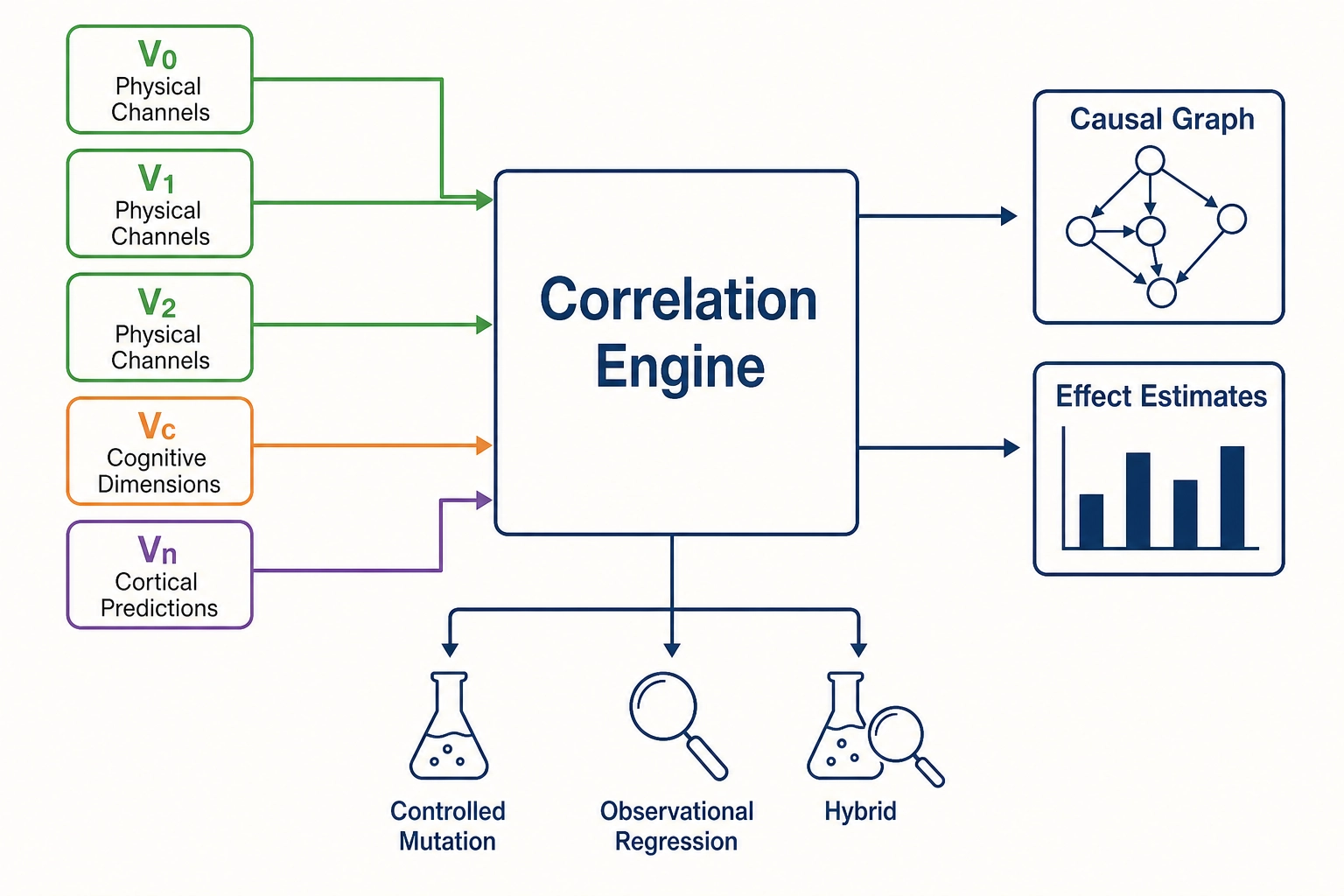
The correlation engine answers one question in many forms: when a content property changes, what happens to the viewer’s behavior?
The content property can be physical - the mean linear luminance of a video (V₀), the cut rate in cuts per second (V₁), the pacing acceleration over the file’s duration (V₂). It can be cognitive - the fraction of frames containing a face (Vc), the narrative arc position (Vc), the predicted emotional valence (Vc). It can be cortical - the predicted mean activation of the fusiform face area (Vₙ), the predicted visual-network engagement (Vₙ).
The behavioral outcome is always Vₚ: average view duration, completion rate, engagement rate, share rate, comment volume, follower conversion - the twenty-two platform metrics that Chapter 6 specified. For each content property and each Vₚ outcome, the correlation engine estimates a relationship: how much does this outcome change when this property changes by a given amount? The estimate comes with a confidence interval, a workflow tag (was the evidence experimental or observational?), a persona tag (for which viewer group does this hold?), and a Vc-Vₙ consistency flag (did the cognitive and cortical approximations agree on the content property?).
The engine produces not a single number but a structured record - an edge in a graph - carrying enough metadata for a downstream consumer to evaluate evidence quality, generalizability, and mechanistic plausibility. Over time, the collection of edges becomes a growing causal graph.
What the engine does not do is equally important. It can infer which aspects of cortical processing were engaged (from Vₙ), how strongly, and how independently. It cannot infer the subjective quality of that processing. The which / how-strongly / how-independently / never-what-it-feels-like discipline from Chapter 5 applies without modification. What the viewer actually felt remains structurally opaque, accessible only through the self-report data that Chapter 6 introduced.
2. Statistical Methodology
The correlation engine does not commit to a single statistical technique. It commits to a vocabulary of regression families and a decision procedure for selecting among them. The choice depends on the hypothesis being tested and the structure of the data.
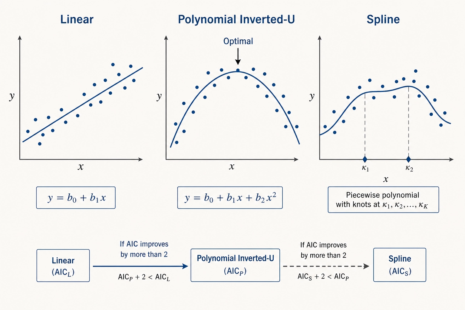
Linear models as the default
The starting point is a linear model. The reason is interpretability: the coefficient on the target variable is directly readable as the expected Vₚ change per unit change in the content property. “A 10-percentage-point increase in face-area fraction is associated with a 1.8-second increase in average view duration” is a statement a content creator can act on.
The interpretability advantage comes with a trade-off: linear models assume the effect is constant across the full range of the property, which may not hold (section 2’s non-linear models address this when it does not). Three linear forms are available. Ordinary least squares (OLS - the standard regression technique that fits a line by minimizing the sum of squared residuals) for continuous Vₚ outcomes like average view duration. Logistic regression for binary outcomes like completed-versus-not-completed. Poisson or negative-binomial regression for count outcomes like comment volume, where overdispersion (the variance exceeding the mean, common in count data) is present.
Non-linear models when the data warrants them
Some content properties have theoretical reasons for non-monotonic relationships with outcomes. Pacing is a clear example: too slow is boring, too fast is overwhelming, somewhere in the middle is engaging. Luminance variance, audio energy, and visual complexity are similar - the inverted-U relationship between stimulus intensity and engagement has been theorized since the psychologist Daniel Berlyne (1960), who proposed that moderate novelty and moderate complexity produce the strongest positive response, with both extremes (too simple, too complex) producing weaker engagement. The marketing researchers Jianhua Shi, Chengqi Li, and Pattharin Chumnumpan (2025) provide a direct bridge from Berlyne to short-form video, finding an inverted U-shaped relationship between auditory arousal and engagement across 12,842 short-form videos [10].
When the linear model shows systematic residual structure - curvature in the residual-versus-fitted plot - the correlation engine fits a non-linear alternative. Two forms are committed. First, polynomial terms: adding a squared term for the target variable tests for inverted-U or U-shaped relationships. Second, restricted cubic splines with three to five knots (a flexible curve-fitting technique that bends at specified data points without overfitting), placed at quantiles of the target variable’s distribution, for relationships whose shape is unknown in advance.
The decision rule is mechanical: if the linear model’s AIC (Akaike Information Criterion - the standard model-comparison metric that balances fit against complexity) is lower than the non-linear model’s AIC by more than 2 units, the linear model is retained. Otherwise, both models are reported with their AIC values and effect estimates, and the analyst inspects which one better describes the data.
Interaction models
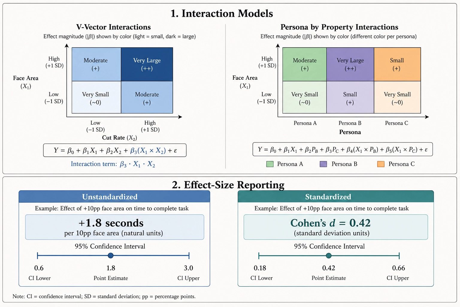
Some relationships depend on context. Does the effect of face area on retention depend on cut rate? Does the effect of luminance variance on engagement differ between personas? Interaction models test these conditional relationships by including product terms - the target property multiplied by the moderating variable - in the regression.
Two forms of interaction are tested. V-vector interactions test whether one content property’s effect depends on another content property. Persona-by-property interactions test whether a content property’s effect differs across viewer segments. Only pre-registered interactions are tested; exploratory interactions discovered after the fact are flagged as hypothesis-generating, not hypothesis-confirming.
The engine tests two-way interactions only in v1. Three-way and higher interactions - does the effect of face area depend on cut rate and persona simultaneously? - require substantially larger sample sizes to detect reliably, and Khozai’s experiment scale (hundreds of experiments, not billions of observations) will not support them.
Effect-size reporting
Every effect estimate the correlation engine produces is reported in two forms. The unstandardized coefficient gives the effect in the natural units of both variables - seconds of view duration per percentage point of face area, for instance. This is the operationally useful number. The standardized coefficient gives the effect in standard-deviation units (Cohen’s d for experimental comparisons, partial eta-squared for regression contexts), enabling comparison across dimensions and outcomes that have different natural scales.
Every estimate carries a 95% confidence interval - from the regression’s standard-error estimate for linear models, from bootstrap resampling with 1,000 iterations (bootstrap - repeatedly re-sampling the data with replacement to build an empirical distribution of the estimate) for non-linear and interaction models. The confidence interval is the primary inferential tool. P-values are reported for compatibility with statistical convention but are secondary.
Effects whose confidence interval includes zero are reported as “not distinguishable from zero at the 95% level.” They are stored and contribute to meta-analytic aggregation, but they are not reported as positive findings. Effects whose interval excludes zero but whose magnitude falls below a minimum operationally meaningful threshold - set per Vₚ outcome in Chapter 10’s calibration process - are reported as “statistically detectable but below operational relevance.” Less than half a second of average view duration, for example, may be detectable with a large sample but irrelevant to a content creator.
Multiple-testing correction
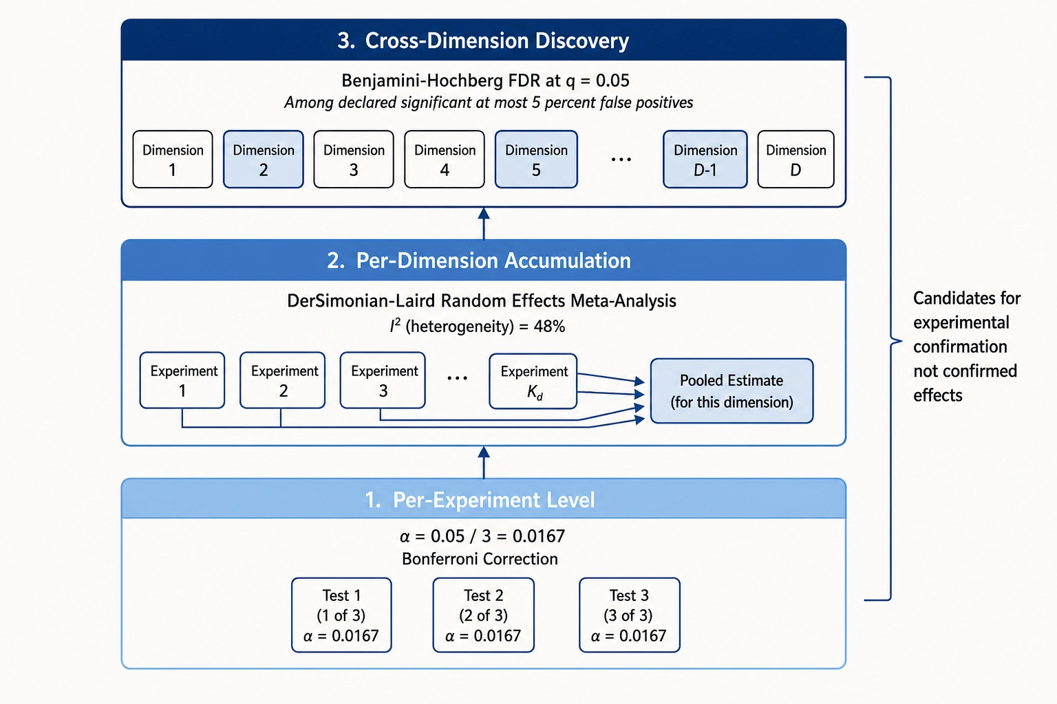
The correlation engine tests many hypotheses across many V-vector dimensions, many Vₚ outcomes, and many personas. Without correction, the false-positive rate would be unacceptable. The correction strategy is hierarchical, matching the V-vector architecture.
At the per-experiment level, Bonferroni correction (dividing the significance threshold by the number of tests) is applied within the experiment’s test set. With three Vₚ outcomes, the threshold becomes α = 0.05 / 3 = 0.0167.
At the per-dimension accumulation level, as experiments accumulate for the same content dimension, the engine aggregates effect estimates using a random-effects meta-analytic framework (DerSimonian-Laird estimator - the standard method for pooling effect sizes that allows for between-study variance). Significance is assessed on the pooled estimate, not on individual experiments.
At the cross-dimension discovery level, when observational regression scans across multiple V-vector dimensions simultaneously, the false discovery rate is controlled using the Benjamini-Hochberg procedure at q = 0.05 - among all dimensions declared significant, at most 5% are expected to be false positives. FDR-controlled results are candidates for experimental confirmation, not confirmed effects.
3. Causal Identification - Khozai’s Way
Correlation is not causation. The phrase is a cliche because it names a real problem. A video with warm colors and high retention may owe its retention to the narrative, the creator’s audience, or the publication timing - not to the colors. Separating the property that matters from everything else that varies is the problem of causal identification. Khozai addresses it with three native workflows, each with a different causal-identification strategy, a different data source, and a different confidence ceiling.
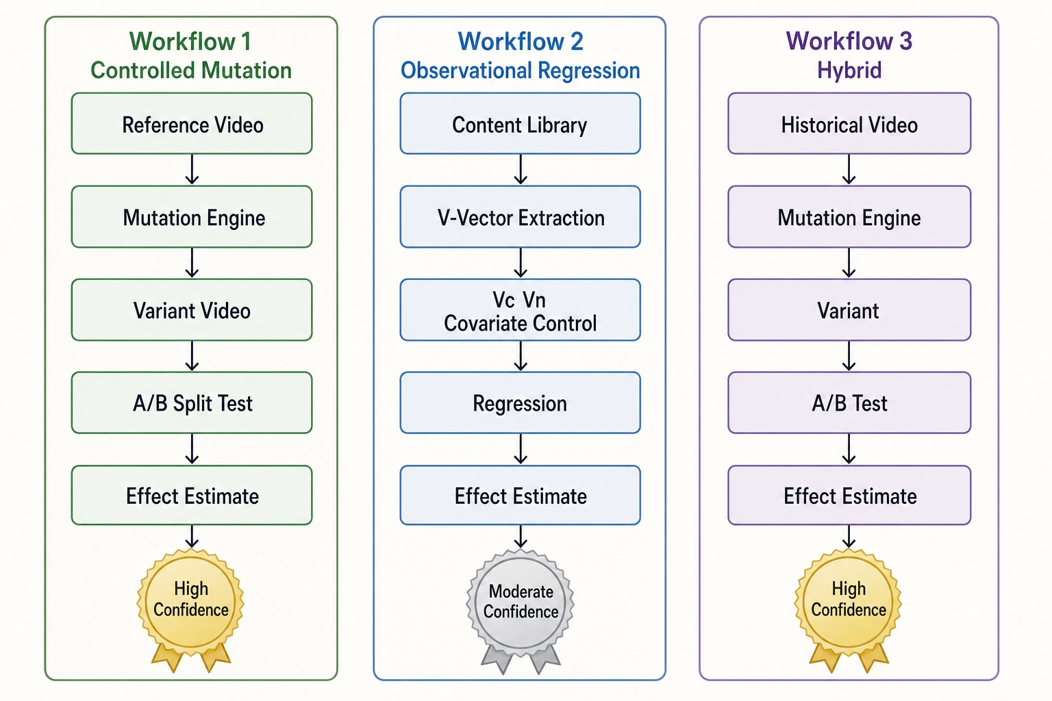
Workflow 1: Controlled mutation
The gold standard. The mutation engine (Chapter 7) generates a reference version and a variant that differ by a single operator application. The V∆ between them is measured by the verification pipeline before publication. The Vₚ difference is measured after publication under identical conditions - same budget, same pacing, same account, same optimization target, same audience randomization.
Causal identification comes from the experiment itself, not from statistical adjustment. The experimenter controlled the independent variable (the operator application) and randomized the assignment (the platform’s split-test product assigns impressions server-side). This is the same logic that governs any controlled experiment in science: change one thing, hold everything else constant, measure the effect. The regression’s role in workflow 1 is to estimate the magnitude and precision of the effect, adjusting for residual noise (posting-time effects, day-of-week effects, account-follower-count drift between experiments). It is not to identify the cause - the cause was identified by the experimental design.
Confidence ceiling: high. Bounded by the quality of the isolation (how well the operator held non-target dimensions constant, as verified by the four-layer verification pipeline) and the statistical power of the experiment (sample size relative to the effect size, per the Phase-7 experimental design defaults - significance level α = 0.05 two-sided, power 0.80, minimum detectable effect of a 5% relative shift).
Workflow 2: Vc/Vₙ-controlled regression on existing content libraries
Not every question can wait for a controlled experiment. When Khozai has access to a library of existing content - the creator’s own archive, a competitor’s public catalog, a curated dataset - it can learn from the variation that already exists. The problem is confounding: existing videos differ on dozens of properties simultaneously. A video with high luminance variance (V₀) might also feature dramatic scene changes (Vc) and strong visual-cortex activation (Vₙ). Without separating these correlated properties, the regression cannot attribute the behavioral outcome to any one of them.
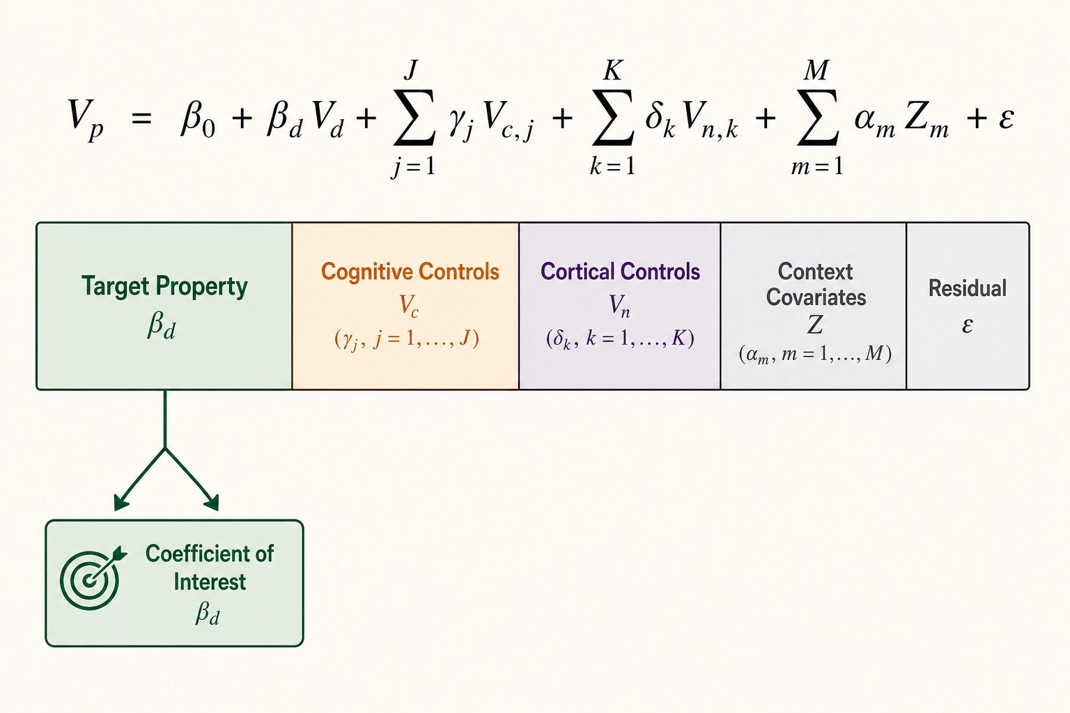
Khozai’s native solution is to use its own vector architecture as the confounder control. The formal regression structure for a single physical dimension d is:
Vₚ_outcome = β₀ + β_d · V_d + Σⱼ(γⱼ · Vcⱼ) + Σₖ(δₖ · Vₙₖ) + Σₘ(αₘ · Zₘ) + ε
where Vcⱼ are the thirty-two Vc dimensions, Vₙₖ are the Vₙ aggregates (Glasser-360 parcels aggregated to Yeo-7 or Yeo-17 network-level mean activations), Zₘ are context covariates from the Vₚ specification (platform, posting time, account follower count, paid promotion flag, content duration), and ε is the residual. The coefficient of interest is β_d - the association between the target physical property and the behavioral outcome, net of everything Vc and Vₙ capture.
This workflow is native to Khozai in a specific sense: Vc and Vₙ are already computed for every video in the corpus. They are the framework’s own cognitive and cortical approximations - each confounder dimension has a defined meaning (“fraction of frames with a face present,” “predicted mean fusiform-face-area activation”) - and the researcher can inspect, interpret, and challenge the controls. No external covariate set, no separate nuisance model.
The confidence ceiling is moderate. The association is causal only to the extent that Vc and Vₙ capture all relevant confounders - and they do not capture three categories. First, unobserved audience characteristics: two videos may differ in Vₚ because they reached different audiences. Second, temporal and cultural context: a video published during a trending moment performs differently from the same content at a quieter time. Third, algorithmic recommendation effects: the platform amplifies or suppresses distribution based on early engagement, making Vₚ partly a function of the platform’s response to early Vₚ.
Effects discovered in workflow 2 are candidates for experimental confirmation in workflow 1, not causal conclusions by themselves.
Workflow 3: Hybrid
The hybrid workflow combines observational grounding with experimental causal identification. Pick a historical video - one the creator already published, with known V-vectors and already-observed Vₚ - and use it as the reference for a controlled mutation. Apply an operator to its scene-AST representation, verify through the four-layer pipeline, publish the variant, compare outcomes.
The hybrid inherits the causal-identification strength of workflow 1 (controlled, randomized mutation) while starting from a reference with ecological validity (a real video that performed in the real world). At Khozai’s operating scale - hundreds to thousands of experiments, not billions of impressions - starting from content with demonstrated engagement gives each experiment more leverage than starting from a synthetic baseline.
Confidence ceiling: high for the forward-mutation component. The historical video’s Vₚ provides a behavioral anchor - “what happens when I change one property from this known baseline?” - rather than “does this synthetic video work at all?”
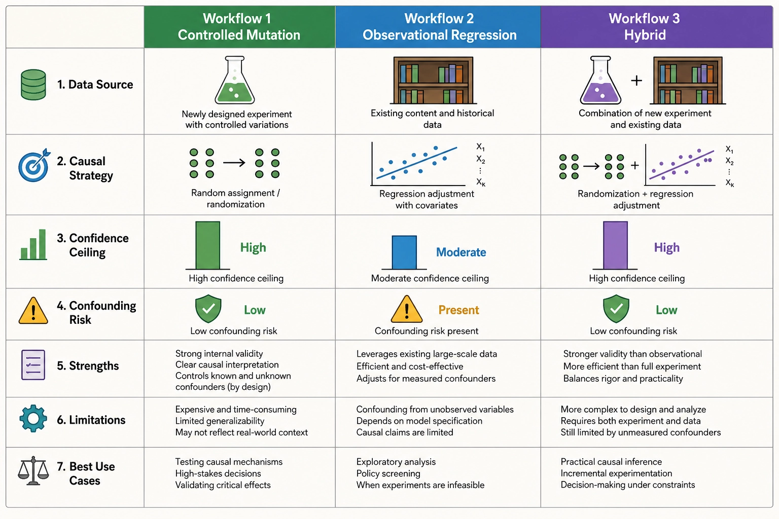
Comparison of causal-identification workflows
| Dimension | Workflow 1: Controlled mutation | Workflow 2: Vc/Vₙ-controlled regression | Workflow 3: Hybrid |
|---|---|---|---|
| Data source | New experiment (reference + variant) | Existing content library | Historical video + new variant |
| Causal-identification strategy | Randomized controlled experiment | Statistical control via Vc and Vₙ covariates | Randomized mutation from ecological baseline |
| Counterfactual generation | Scene-AST operator with verified isolation | Natural variation in corpus | Scene-AST operator applied to real video |
| Confidence ceiling | High | Moderate | High (forward-mutation component) |
| Residual confounding risk | Low (bounded by isolation quality) | Present (unobserved audience, timing, algorithmic effects) | Low for mutation delta; baseline inherits observational limits |
| Minimum data requirement | One experiment per property-outcome pair | Large corpus with sufficient property variance | One historical video + one experiment |
| Primary use case | Confirming causal effects | Screening candidates for experimental confirmation | Grounding experiments in ecologically valid content |
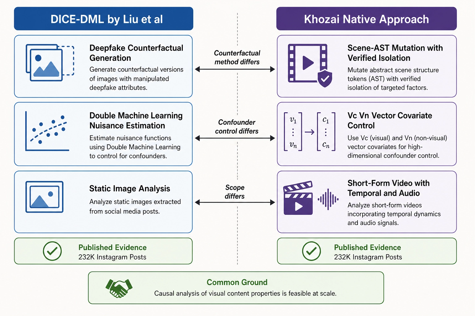
Adjacent landscape: Liu et al. and DICE-DML
Khozai’s three workflows are not the only approach to causal analysis of visual content properties. Published work in the adjacent space provides evidence that the general approach - measuring content properties and estimating their effects on engagement outcomes - is feasible and productive.
The econometricians Yang Liu, Karthik Padmanabhan, and Madhu Viswanathan, “Estimating Visual Attribute Effects in Advertising from Observational Data: A Deepfake-Informed Double Machine Learning Approach,” published as a research paper on arXiv (arXiv:2603.02359, submitted March 2, 2026), demonstrate one such approach. Their method, DICE-DML, uses deepfake-generated counterfactual images paired with originals, then applies double machine learning (DML - a statistical framework that uses ML models to estimate nuisance parameters while preserving valid causal inference, NCJ) to estimate the effect of visual attributes - face presence, text presence, color features - on engagement metrics across 232,089 Instagram influencer posts, reporting 73 to 97 percent RMSE reduction versus standard DML in simulation.
This is green-flag evidence. The paper confirms that the general question the correlation engine asks - “what is the causal effect of this visual property on this behavioral outcome?” - is answerable at scale in the advertising domain. It is published evidence that the approach works, making Khozai’s ambition less speculative. It is not proof that Khozai’s specific approach will succeed, but evidence that the domain supports this kind of analysis.
Khozai does not adopt the DICE-DML methodology. Three differences drive the divergence. First, counterfactual generation: DICE-DML uses deepfake techniques relying on the generative model’s ability to change one attribute without changing others; Khozai uses its scene-AST mutation engine with structurally declared and verified isolation. Second, confounder control: DICE-DML uses DML’s flexible nuisance-parameter estimation; Khozai workflow 2 uses its own Vc and Vₙ vectors - less flexible but more interpretable, requiring no additional model training. Third, scope: DICE-DML operates on static images; Khozai operates on short-form video with temporal dimensions, audio channels, and cortical-temporal dynamics.
Khozai cites DICE-DML as evidence that causal analysis of visual content properties is valid. The methodology Khozai adopts is native to its own vector architecture.
4. Population Segmentation - Personas
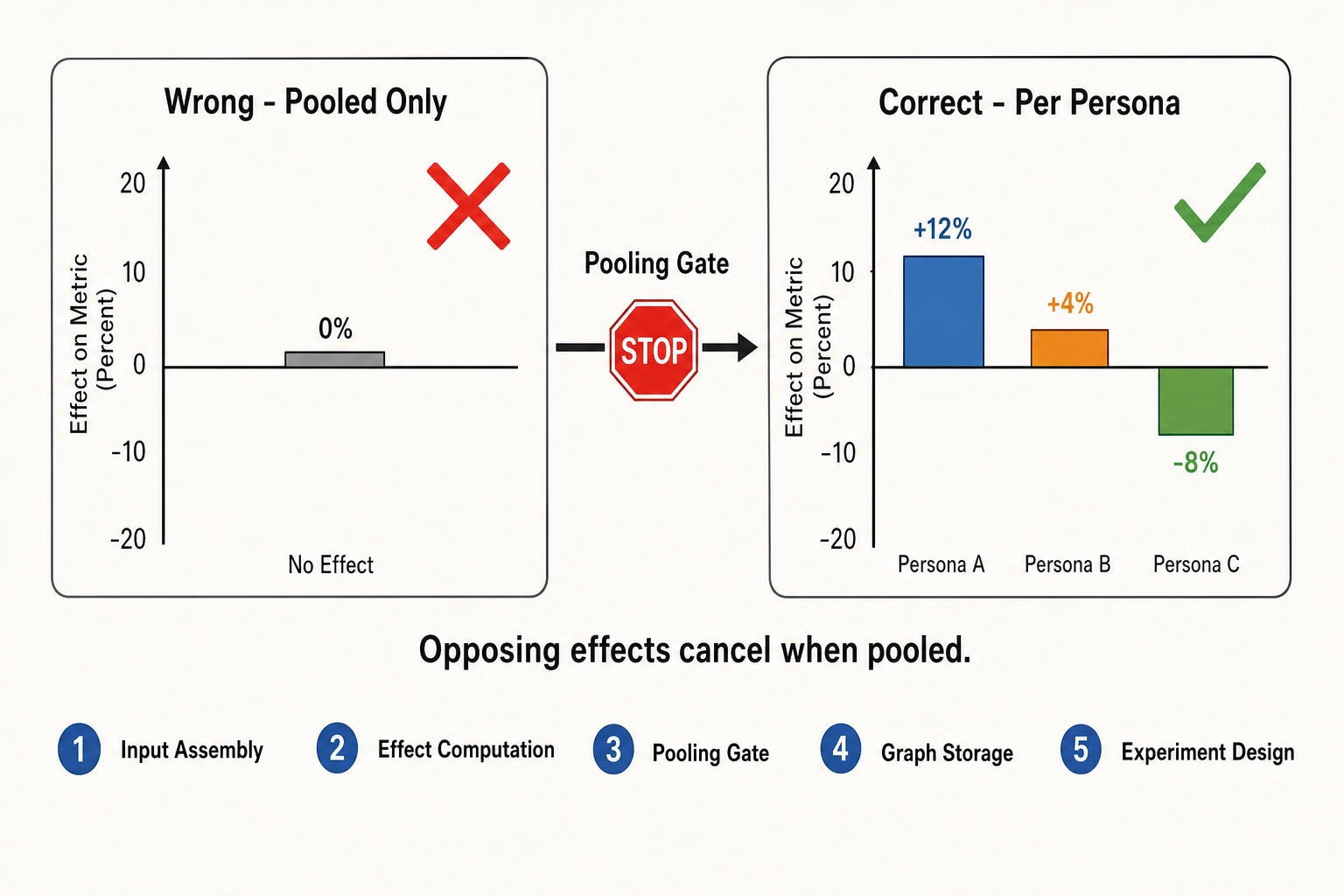
A mutation that increases retention for one group of viewers may decrease it for another. If those groups are collapsed into a single population, the opposing effects cancel, the correlation engine reports no effect, and the framework draws the wrong conclusion. This is not a hypothetical concern - it is a structural feature of any content system that serves heterogeneous audiences.
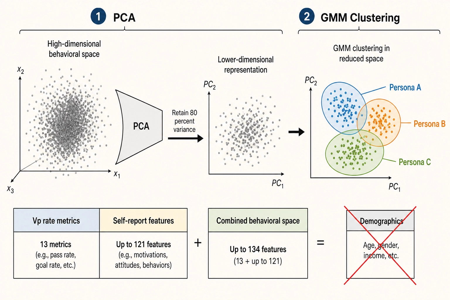
Khozai’s mechanism for preventing this collapse is the persona: a behaviorally defined cluster of viewers who respond to content in similar ways. Not a demographic bracket (age, gender, geography), not a psychographic label (“adventurous millennials”), not a marketing archetype - a pattern in what viewers actually do and report, discovered from the data and validated by its ability to separate effect sizes that would cancel if pooled.
How personas are defined
Personas are constructed from two data sources. From the Vₚ side: thirteen platform metrics expressed as rates - view-through rate, fraction-watched, completion rate, four quartile retention values, replay rate, like rate, comment rate, save rate, share rate, and follower-conversion rate per thousand views. From the self-report side: up to 121 features - activation rates and magnitudes for experiential dimensions at Resolution Levels 1 and 2, Scope B tag frequencies, and construct-confirmation match rates for the four locked constructs (anxiety, flow, nostalgia, awe). No demographic variable enters the clustering input. Demographics may correlate with behavioral clusters, but the correlation is noted as observation, never as definition.
The unit of analysis is the viewer-content pair. A viewer who laughs at comedy and cries at a memorial is expressing two different response patterns; persona is a property of a response, not of a person.
The clustering method is a two-stage pipeline. First, PCA (principal component analysis - the standard technique for reducing high-dimensional data to fewer orthogonal components capturing the most variance) reduces the feature set to the components explaining at least 80% of total variance. Second, Gaussian Mixture Model clustering (GMM - a method that models each cluster as a probability distribution, producing soft assignments rather than the hard boundaries of K-means) is applied to the reduced space. This PCA-plus-clustering approach on behavioral interaction data has been validated for user segmentation by the information systems researcher José Vargas-Calero and colleagues (2025) [11]. The number of clusters K is selected by BIC minimization (Bayesian Information Criterion - the standard model-selection metric that penalizes complexity) across K = 2 through K = 15. The upper bound is practical: each additional persona multiplies the minimum experiment size.
Persona-construction methodology
| Step | Operation | Detail |
|---|---|---|
| 1. Feature assembly | Collect Vₚ behavioral rates and self-report features | 13 Vₚ rate metrics + up to 121 self-report features; no demographic variables |
| 2. Unit definition | Define unit of analysis as viewer-content pair | A single viewer contributes multiple response patterns across different content |
| 3. Dimensionality reduction | PCA on combined feature set | Retain components explaining at least 80% of total variance |
| 4. Clustering | GMM on reduced space | Test K = 2 through K = 15; select K by BIC minimization |
| 5. Validation | Confirm persona utility | Verify that per-persona effect sizes separate effects that cancel when pooled |
The never-collapse rule
The never-collapse-across-personas rule is the operational expression of a design constraint. It is enforced at five specific points in the analysis pipeline.
Point 1: Input assembly. When the correlation engine assembles a dataset for analysis, persona assignment is a mandatory covariate or stratification key. A regression that omits persona fails the pipeline’s input-validation check.
Point 2: Effect-size computation. Effect sizes are computed per persona first. The per-persona estimates are the primary output. A pooled estimate is secondary and derived.
Point 3: Pooling gate. Before a pooled estimate is reported, a heterogeneity test checks two conditions: all per-persona effects must be in the same direction (sign consistency), and the ratio of the largest to the smallest per-persona effect must be below a threshold (magnitude compatibility, set in Chapter 10’s calibration). If either condition fails, the pooled estimate is suppressed and replaced with a per-persona breakdown. Until Chapter 10 lands the threshold, the default is conservative: any sign inconsistency blocks pooling.
Point 4: Causal-graph storage. Effect sizes are stored per persona in the causal graph. A query for an unpersonaed scalar triggers a warning and applies the pooling gate.
Point 5: Experimental design. Mutation experiments must recruit enough viewers to achieve target statistical power within each persona cluster, not merely across the pooled population. The minimum viable experiment size scales with persona count.
The rule does not prohibit reporting a population-level effect alongside per-persona effects. It prohibits reporting only the population-level effect when persona-level heterogeneity exists. A population-level null result may mask a genuine positive effect in one persona canceled by a genuine negative effect in another. That discovery - the opposing effects - is one of the primary analytical payoffs of the persona layer.
A known limitation: behavioral clustering on viewer-content pairs may produce personas that are artifacts of content-type confounding rather than genuine behavioral segments. If a creator’s library is dominated by two genres, the clustering may separate genre-preference groups rather than response-style groups. Cross-content-type validation (testing whether the same personas emerge on held-out content types) is required before treating persona definitions as stable.
5. The Cumulative Causal Graph
The correlation engine does not produce a single report. It produces a growing data structure - a causal graph - that accumulates everything the engine has learned across all experiments, all observational analyses, and all personas.
Nodes
The graph contains three types of nodes.
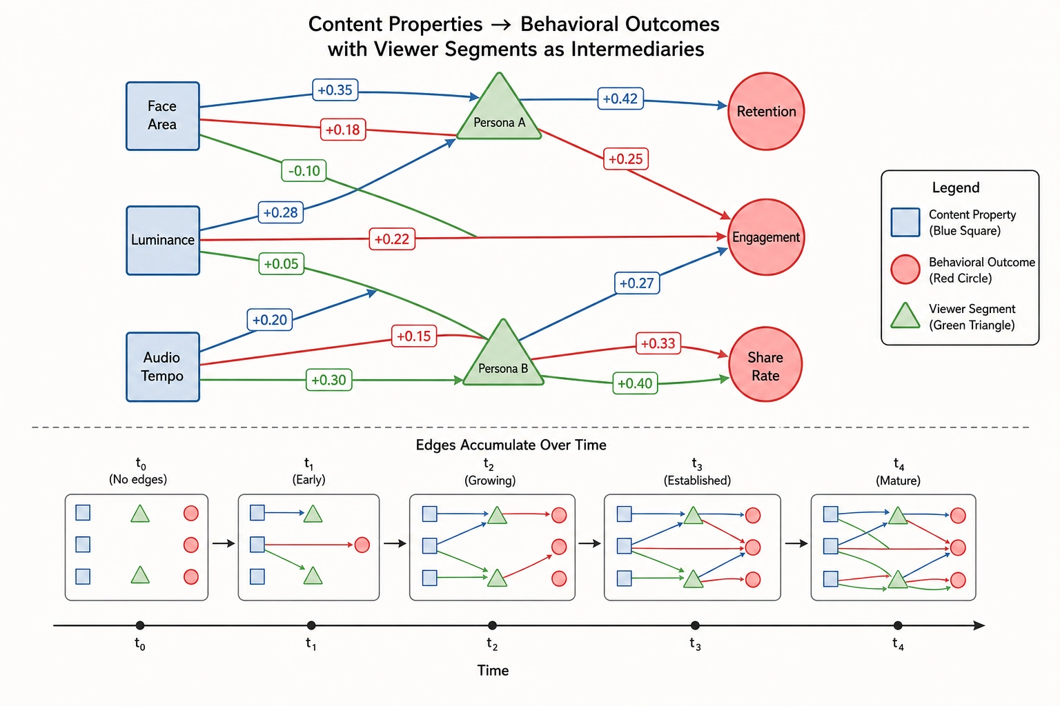
Property nodes represent content properties - specific V-vector dimensions at specific layers. Each node carries a layer tag (V₀, V₁, V₂, Vc, Vc-temporal, or Vₙ), a dimension name from the Phase 3 specifications, a space assignment (Physical Stimulus Space or Neural State Space), and a plain-language description.
Outcome nodes represent behavioral outcomes - specific Vₚ metrics. Each carries a metric name, a Behavioral Output Space assignment, and a description.
Persona nodes represent viewer personas as defined in section 4. Each carries a persona identifier, a description, and the persona-specification version under which it was defined.
Edges
Every edge connects a property node to an outcome node, optionally scoped to a persona node. It carries the full evidentiary record: effect sizes (unstandardized and standardized) with 95% confidence intervals, p-value, observation or experiment count, replication count, source experiment identifiers, workflow tag, regression family, pre-registration status, FDR-correction status, verification quality from the mutation pipeline, the Vc-Vₙ consistency tag (section 6), the Tool 11 mapping characterization (section 7), the Tool 8 feedback-loop classification (consumed by Chapter 9), and a timestamp.
The graph is not a single flat structure. It is a family of subgraphs indexed by persona. Every edge with a persona tag belongs to that persona’s subgraph. Edges with no persona tag belong to the pooled subgraph, which contains an effect only when the pooling gate (section 4) has justified aggregation. This structure enforces the never-collapse rule at the storage level: a consumer querying the graph for a property-to-outcome relationship receives persona-specific estimates by default and pooled estimates only when homogeneity has been verified.
Accumulation and versioning
Edges accumulate over time. New records are added with timestamps; historical records are never overwritten. The graph at any point in time can be reconstructed by filtering records up to that timestamp - supporting the framework’s self-correcting philosophy.
Per-dimension aggregation uses the DerSimonian-Laird random-effects meta-analytic model. For a given (property, Vₚ outcome, persona) triple, all contributing records are pooled with weights inversely proportional to within-study variance plus between-study variance. The aggregated record includes the pooled effect estimate and its confidence interval, the I² heterogeneity statistic (the percentage of total variation due to genuine heterogeneity rather than sampling error), and the contributing experiment list.
6. Vc-Vₙ Consistency as Confidence - Operationalized
Chapter 5 section 8 introduced the consistency check between Vc and Vₙ: when two independent approximations of the same brain agree on a content property, confidence in both rises; when they disagree, both are flagged. This section operationalizes that principle within the correlation engine - specifying how agreement is defined, how it weights the analysis, and what disagreement triggers.
Agreement definition
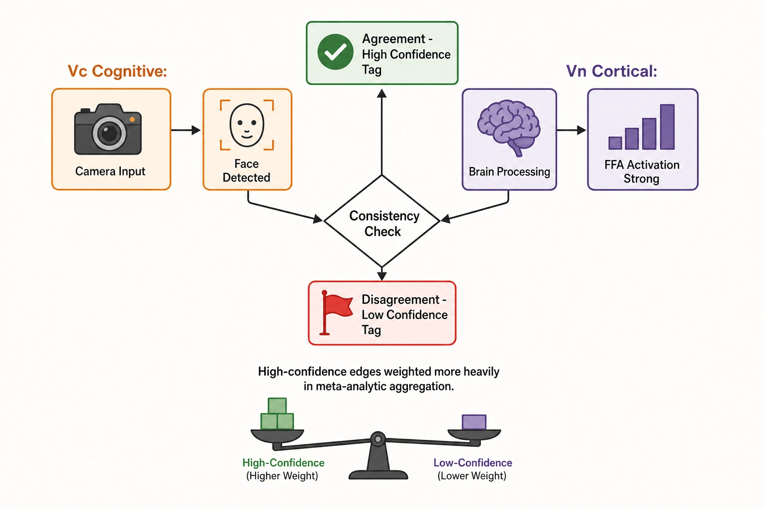
For each content property involved in a correlation, the engine checks whether Vc and Vₙ independently agreed on the relevant content feature.
When the content property is a Vc dimension - face present, for example - the engine checks whether the corresponding Vₙ activation in the expected cortical area is above a threshold indicating strong activation. If Vc reports a face and Vₙ predicts strong fusiform face area (FFA - the cortical region with dedicated neural machinery for face processing) activation, the two agree. If Vc reports a face and Vₙ predicts no FFA shift, they disagree.
When the content property is a V₀, V₁, or V₂ dimension - luminance variance, for example - agreement is assessed on the downstream cognitive and cortical consequences. The engine checks whether Vc identified high visual complexity (a cognitive consequence of luminance variance) and whether Vₙ predicted strong early-visual-cortex activation (a cortical consequence). Agreement here is indirect - it passes through the expected perceptual consequences of the physical property - but it is still informative because the check runs on two independent models.
The specific activation thresholds that define “strong” are set during Chapter 10’s calibration process. This chapter establishes the mechanism; the numbers are locked where they are consumed.
Confidence weighting
Correlations where Vc and Vₙ agree on the content property receive a high confidence tag on their edge record. Correlations where they disagree receive a low tag. In the correlation engine’s analysis, high-confidence edges receive higher analytical weight - they contribute more to the meta-analytic aggregation, and they are reported with greater prominence. Low-confidence edges are not discarded. They are flagged for investigation, because the disagreement may indicate a model error in Vc, a model error in Vₙ, or a genuine case where the cognitive and cortical representations of a content property diverge in a way the framework has not yet accounted for.
The practical effect is that the engine’s knowledge grows faster and more reliably in regions of the content-property space where Vc and Vₙ agree. A face-area effect supported by both the vision-language model’s face detection and the brain encoding model’s FFA prediction accumulates evidence more quickly than a luminance-variance effect where the downstream cognitive and cortical checks are ambiguous. This weighting follows from the architecture’s design assumptions rather than being an independent parameter choice: the framework invests more analytical confidence where it has more independent corroboration.
A limitation of this weighting: it creates an attentional bias toward content properties where Vc and Vₙ happen to overlap well (faces, speech, scene categories) and against properties where one model is weaker (subtle audio features, temporal dynamics). Properties in low-agreement zones may be genuinely important but will accumulate evidence more slowly, potentially delaying discovery of effects that lack a clean cognitive-cortical pairing.
What disagreement does not mean
Disagreement between Vc and Vₙ does not mean the correlation is wrong. It means the evidence is weaker. A face-area mutation that increases retention by 12% is a real observation whether or not Vc and Vₙ agree on the face detection. What the disagreement changes is the framework’s confidence in the mechanistic explanation - the pathway from content property through cortical processing to behavioral outcome. If the cognitive and cortical approximations do not agree on the content property, the mechanistic interpretation (section 8) is less grounded, and the effect should be replicated before it is treated as robust.
7. Tool 11 - Mapping Characterization Applied
Chapter 2 defined Tool 11 (Mapping Characterization) as the formal operation for determining the properties of a mapping between spaces. The correlation engine discovers relationships between content properties (Physical Stimulus Space and Neural State Space) and behavioral outcomes (Behavioral Output Space). Each discovered relationship is a specific instance of a cross-space mapping, and Tool 11 classifies it along five axes.
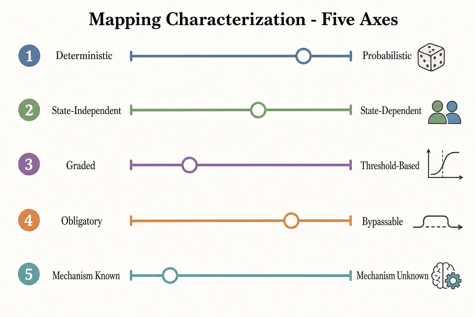
The five axes
Axis 1: Deterministic or probabilistic. Does the same content property value always produce the same behavioral outcome, or does it produce a distribution of outcomes? In practice, every property-to-outcome relationship the correlation engine discovers is probabilistic. The same face-area fraction produces different retention outcomes on different videos, different platforms, and different audiences. The classification is not binary - it is a matter of degree, captured by the width of the confidence interval and the R² of the regression. A narrow interval and high R² indicate a relationship closer to the deterministic end; a wide interval and low R² indicate high stochasticity.
Axis 2: State-dependent or state-independent. Does the relationship depend on the viewer’s current state, or does it hold regardless? The persona dimension of the causal graph provides evidence on this axis. If the effect of face area on retention is +12% for persona A and −3% for persona B, the relationship is state-dependent - the effect depends on which behavioral cluster the viewer belongs to. If the effect is +12% ± 2% across all personas, it is closer to state-independent. The pooling gate (section 4) enforces the measurement: per-persona effects are always computed first, and state-dependence is diagnosed from the heterogeneity test.
Axis 3: Graded or threshold-based. Does the outcome change continuously with the property, or does it jump at a critical value? The regression family selection (section 2) provides evidence. A linear model with a significant coefficient indicates a graded relationship. A spline model with a sharp inflection point, or a polynomial model with a minimum or maximum at a specific property value, indicates a threshold or an optimum. Berlyne’s (1960) inverted-U theory predicts threshold-based relationships for stimulus complexity and arousal - and if the data confirm an inverted-U, the relationship is classified as threshold-based with the optimum noted.
Axis 4: Obligatory or bypassable. Does the content property always affect the outcome, or can the brain’s processing bypass it? The evidence comes from the correlation itself: if a content property shows a significant effect in most experiments but no effect in specific contexts, the mapping may be bypassable in those contexts. Chapter 2 section 3.4 noted that Mapping 4 (Neural State Space to Behavioral Output Space) can bypass Experience Space entirely - reflexes, blindsight, implicit processing produce behavior without conscious experience. A property-to-outcome relationship that bypasses conscious experience would show up as a V₀-to-Vₚ effect without a corresponding Vₙ shift (the cortical-activation intermediary is absent). Tool 8 (Feedback Loop Test), consumed by Chapter 9, classifies these cases as bypass-mediated.
Axis 5: Mechanism known or unknown. Can the pathway from content property to behavioral outcome be traced through a known neuroscience mechanism, or is the correlation empirical without a mechanistic explanation? This is the axis where Vₙ does the most work. When a face-area increase produces stronger predicted FFA activation and higher retention, the mechanism is known: face-area → FFA activation → social-processing engagement → continued watching. When a luminance-variance decrease produces higher completion rate without a clear cortical intermediary, the correlation is real but the mechanism is unknown. The classification is honest - “mechanism unknown” is a valid and frequently used category, not a failure.
Tool 11 mapping axes summary
| Axis | Question | Evidence source | Metric |
|---|---|---|---|
| 1. Deterministic vs. probabilistic | Same input always produces same output? | Confidence interval width, R² | Narrow CI + high R² = more deterministic |
| 2. State-dependent vs. state-independent | Does the effect depend on the viewer’s state? | Per-persona effect heterogeneity | Sign consistency and magnitude ratio across personas |
| 3. Graded vs. threshold-based | Continuous change or jump at critical value? | Regression family comparison (linear vs. spline/polynomial) | AIC comparison; inflection-point detection |
| 4. Obligatory vs. bypassable | Always active or context-dependent? | Cross-context replication | V₀-to-Vₚ effect without Vₙ shift indicates bypass |
| 5. Mechanism known vs. unknown | Traceable cortical pathway? | Vₙ intermediary identification | Named Glasser areas or Yeo networks with known function |
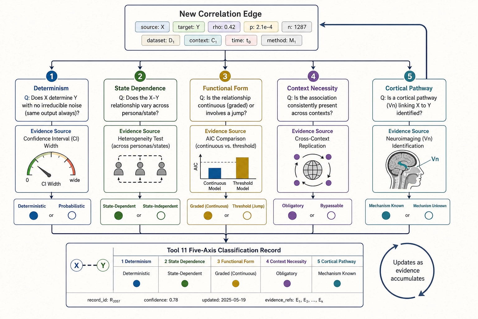
How correlations get classified
Every edge in the causal graph carries a Tool 11 characterization - a five-element record with one value per axis. The classification is not a one-time judgment; it is updated as evidence accumulates. An early correlation may be classified as (probabilistic, unknown-state-dependence, unknown-graded-or-threshold, unknown-obligatory-or-bypassable, mechanism unknown) when it first appears from a single experiment. As more experiments test the same property across different contexts and personas, the state-dependence axis resolves, the graded-versus-threshold axis resolves, and the mechanism axis may resolve if Vₙ provides a cortical intermediary.
The five-axis classification serves two purposes. For the researcher, it communicates what is known and what is uncertain about each relationship. For the framework’s self-correcting process, it identifies where the next experiment should be directed: unknown-mechanism edges need Vₙ-focused analysis; unknown-state-dependence edges need persona-stratified experiments; unknown-graded-or-threshold edges need dose-response designs.
8. Interpretation Through Neuroscience
The correlation engine produces structured relationships - this content property is associated with this behavioral outcome, with this effect size, for this persona, through this workflow. The final step is interpretation: what does the relationship mean? Why does it exist? What is the mechanism that connects a change in pixels to a change in behavior?
This is where Vₙ - the cortical-activation approximation from Chapter 5 - becomes a bridge between statistical association and neuroscience mechanism.
The interpretive chain
Consider the canonical example. A controlled mutation experiment (workflow 1) increases face area from 25% of frame to 55% of frame (using op_face_area with the crop-to-face method). The verification pipeline confirms the target V∆ on face-area fraction and verifies that isolation dimensions (luminance, audio, pacing) stayed within tolerance. The variant is published, and Vₚ data show a +12% increase in average view duration for personas A and B, no significant change for persona C.
The raw finding is: face area +30 percentage points → retention +12% (personas A and B). This is the correlation engine’s output - an edge in the causal graph with effect size, confidence interval, persona tags, and quality metadata.
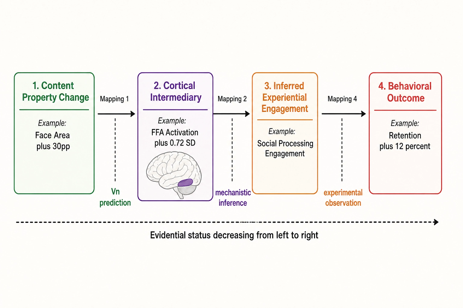
The interpretive step adds the cortical intermediary. Vₙ, re-run on both the reference and the variant as part of the cortical verification layer (Chapter 7 section 4), shows a measurable increase in predicted activation of the fusiform face area - the cortical region where face processing is concentrated. The Vc-Vₙ consistency check confirms agreement: Vc detected a larger face, and Vₙ predicted stronger FFA activation.
The interpretation becomes: larger face → stronger predicted FFA activation → stronger social-processing engagement → continued watching. Each link in the chain has a different evidential status. The first link (larger face → stronger FFA activation) is supported by the Vₙ prediction and by evidence that FFA responses vary parametrically with face size: The vision researcher Xiaomin Yue and colleagues (2011) showed that lower-level stimulus features including face area strongly influence FFA responses, not just the categorical presence of a face [12]. The fusiform face area was identified as a face-selective region by the cognitive neuroscientist Nancy Kanwisher, the psychologist Kathleen McDermott, and the vision researcher Marvin Chun in 1997 [2], and the finding has been replicated extensively. The behavioral link from FFA activation to retention remains an inference: the parametric scaling of FFA with face size is established, but the downstream effect on viewing behavior is what the framework exists to test. The second link (FFA activation → social-processing engagement) is a mechanistic inference - the fusiform face area is part of the brain’s social-processing network, and its activation during content viewing is associated with deeper social cognition. The third link (social-processing engagement → continued watching) is the behavioral observation from the experiment.
What interpretation adds and what it does not
The interpretive step adds mechanistic plausibility - transforming “face area causes retention” from a black-box finding into a claim with a neurological pathway. It tells the content creator not just what to change but why the change works.
What it does not add is certainty. The Vₙ prediction is a model output, not a brain scan. Whether TRIBE v2’s specific prediction for a specific video preserves enough signal for the interpretation to hold is an empirical question - the core of Bet 2. The neuroscience literature confirms the general principle (faces activate FFA), but whether the predicted signal is accurate enough to ground specific interpretations is what the framework exists to test. The interpretation is the best available mechanistic account. It is not a proven causal chain. Furthermore, cortical encoding models like TRIBE v2 are trained on fMRI data from controlled laboratory settings with passive viewing tasks; their predictions may not generalize to the active, distracted, multi-tab viewing conditions typical of short-form content consumption. The degree of generalization is itself an empirical question the framework must test.
A second example: audio tempo and auditory cortex
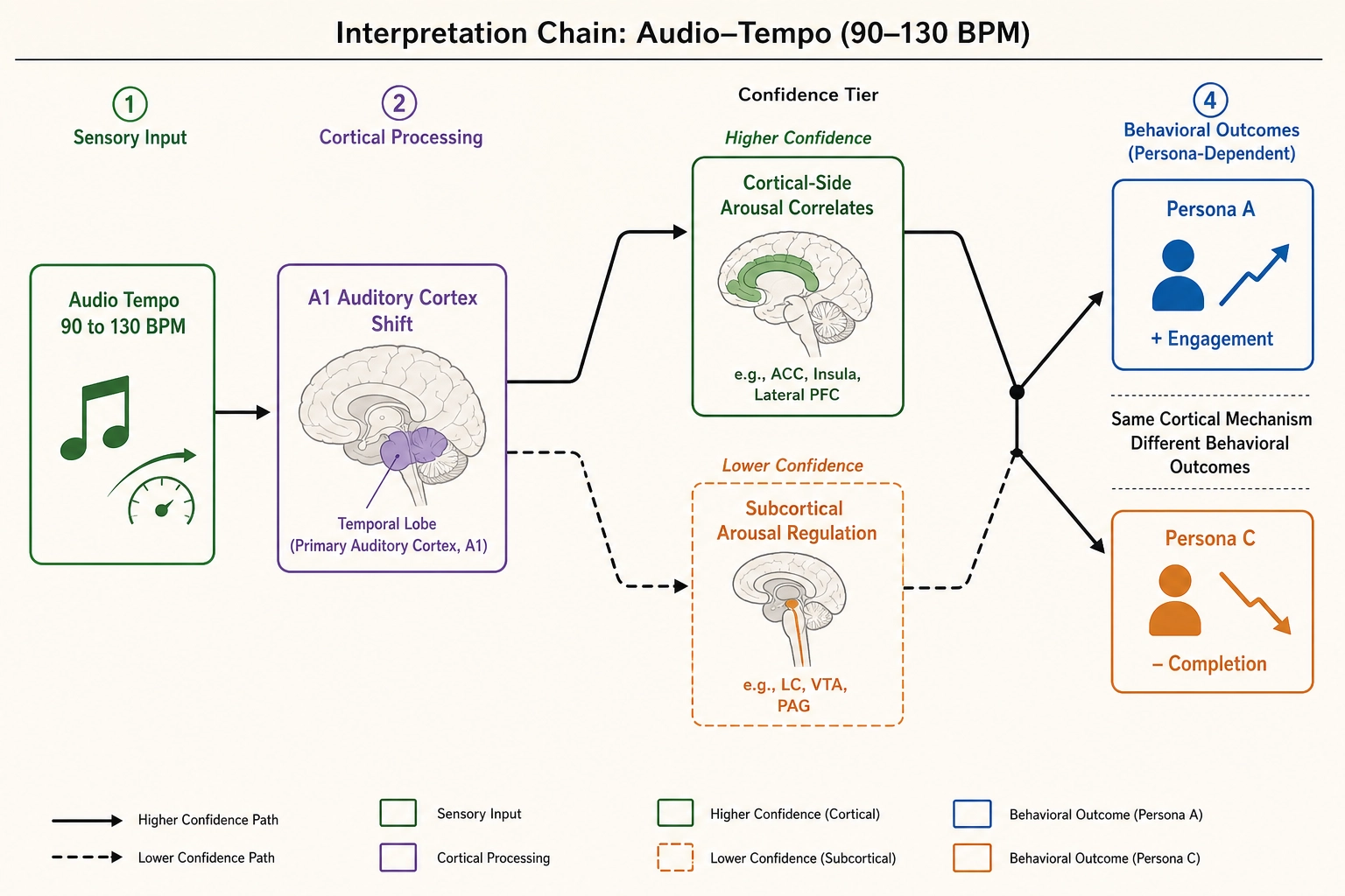
A workflow 1 experiment increases audio tempo from 90 beats per minute to 130 beats per minute using op_time_stretch. Vₙ predicts a shift in the activation pattern of primary auditory cortex (A1 - the cortical region that processes basic auditory features including pitch, rhythm, and temporal patterns) and adjacent auditory association areas. The Vₚ outcome depends on persona: persona A shows increased engagement rate; persona C shows decreased completion rate.
The interpretation for persona A: faster tempo → altered auditory cortex activation pattern → cortical-side correlates of arousal modulation → increased active engagement. The interpretation for persona C: faster tempo → same cortical shift → perceived processing overload → earlier drop-off. The same cortical mechanism produces different behavioral outcomes for different personas - a concrete instance of the state-dependence axis from Tool 11.
An important caveat: arousal itself is regulated by subcortical structures - the brainstem’s reticular activating system and the locus coeruleus. Khozai predicts activation in these subcortical structures with lower confidence than cortical predictions due to fMRI SNR limitations (per Chapter 5 section 6). The subcortical predictions are included because arousal regulation is among the most relevant signals for content engagement - but the confidence differential means that interpretations grounded in subcortical arousal pathways carry less certainty than those grounded in cortical intermediaries. The correlation engine can observe cortical-side correlates of arousal modulation (auditory cortex, the salience network) at higher confidence, and subcortical arousal regulation at lower confidence. The interpretation distinguishes these confidence tiers: “cortical-side correlates of arousal modulation” for higher-confidence claims, “predicted subcortical arousal regulation” for lower-confidence claims.
The interpretive discipline
Every neuroscience interpretation follows a three-part discipline. First, state the cortical intermediary - which Glasser areas or Yeo networks showed a predicted activation shift, in which direction. Second, state the known function - FFA processes faces; A1 processes auditory features; the temporal parietal junction (TPJ - the part of the brain that models other people’s intentions and mental states) processes social cognition, as established by the cognitive neuroscientists Rebecca Saxe and Nancy Kanwisher (2003) [13] and confirmed across paradigms in the neuroscientist Matthias Schurz and colleagues’ (2014) meta-analysis [14]; the default mode network (DMN - the cortical regions active when a person is relating what they see to their own life, imagining what might happen next, or reflecting inward) processes self-reference and imagination [15]. These attributions are grounded in published neuroscience. Third, state the inferential link to the behavioral outcome as an inference, not as a proven mechanism. “Stronger FFA activation → stronger social-processing engagement → continued watching” rests on two testable assumptions: that Vₙ accurately reflects cortical processing (Bet 2), and that cortical processing is the relevant intermediary (investigable through Chapter 9’s feedback-loop classification). Neither is assumed true. Both are the framework’s working hypothesis, and the correlation engine’s accumulating evidence either supports or undermines them.
Khozai can identify the cortical regions involved, estimate their activation magnitude, and assess whether they operate independently of one another. It cannot access the subjective quality of that processing. The fusiform face area activating does not tell us what seeing a face feels like. That is Scope B of Experience Space - structurally opaque, accessible only through self-report, and never claimed by the correlation engine.
The correlation engine turns measurements and experiments into structured knowledge - mapping content properties to behavioral outcomes through three workflows, segmenting the population into personas, accumulating edges into a growing causal graph, weighting confidence by Vc-Vₙ agreement, classifying relationships along Tool 11’s five axes, and interpreting them through cortical intermediaries. Always specifying the cortical regions involved, the magnitude of predicted activation, and the degree of independence between processing streams. Never claiming to know what any of it feels like.
What this does NOT say
Three claims this chapter does not make. First, the correlation engine does not claim causation from observational data alone: workflow 2 produces associations controlled for Vc and Vₙ, not proven causal effects - only workflow 1’s controlled mutations and workflow 3’s hybrid experiments produce causal evidence, and even those are bounded by isolation quality and statistical power. Second, the chapter does not claim that persona clusters are stable across content types: a persona defined on comedy response data may not separate the same viewer groups on documentary response data, and cross-content-type stability is an empirical question the framework must test, not an assumption it can make. Third, the causal graph is not claimed to be complete: it accumulates edges as experiments run, but at any point in time it represents what has been tested, not what exists - unmeasured properties, untested personas, and undiscovered interactions remain outside the graph until experiments bring them in.
Khozai implication
The correlation engine is the point where Khozai’s measurement infrastructure meets its empirical ambition. Chapters 5 through 7 built the instruments: content vectors, viewer vectors, and a mutation engine. This chapter turns those instruments into an analytical system that can ask “what drives what, for whom, with what confidence?” and accumulate the answers into a growing, self-correcting knowledge structure. The 109 content-side channels (V₀: 25, V₁: 16, V₂: 12, Vc: 32, Vc-temporal: 24), the 22 platform metrics, and the persona layer create a combinatorial space of testable hypotheses. The framework does not need to test all of them - it needs to test enough of them, in the right order, to build a causal graph dense enough to guide content decisions. The three workflows give it three speeds: fast observational screening, rigorous experimental confirmation, and ecologically grounded hybrid testing. The Vc-Vₙ consistency check and the Tool 11 classification ensure that each edge in the graph carries not just a number but a quality assessment and a mechanistic interpretation. Khozai’s contribution is not a new statistical method - the regression families, the meta-analytic aggregation, and the FDR corrections are standard. The contribution is the integration: a system where physics-level content properties, cognitive approximations, cortical predictions, behavioral outcomes, and viewer segmentation feed into a single analytical engine that grows more informative with every experiment. Whether this integration adds value beyond what individual components deliver separately is the empirical question the framework exists to answer.
Conclusion
The correlation engine transforms Khozai’s measurement and mutation infrastructure into structured inference - estimating how content properties drive behavioral outcomes, for which viewer personas, through which cortical pathways, at what confidence level. Its three causal-identification workflows provide observational screening, experimental confirmation, and hybrid grounding; its persona layer prevents the collapse of heterogeneous effects into misleading averages; and its cumulative causal graph accumulates evidence across experiments while preserving the metadata needed to evaluate each edge’s quality. The engine’s honesty constraints - never claiming causation without experimental support, never collapsing across personas without verified homogeneity, never claiming to know what cortical activation feels like - are as important as its analytical capabilities.
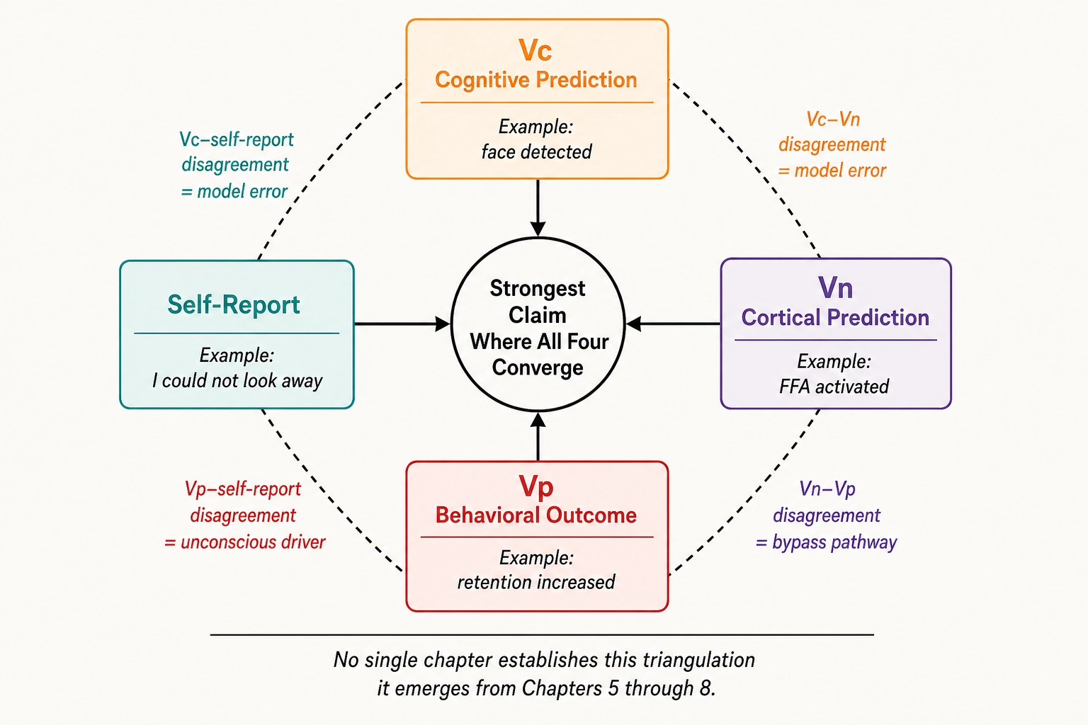
Two architectural consequences emerge from the full pipeline. First, the framework now has four-way triangulation for every claim about content impact: cognitive prediction (Vc says “face detected”), cortical prediction (Vₙ says “FFA activated”), behavioral outcome (Vₚ says “retention increased”), and self-report (viewer says “I couldn’t look away”). Claims are strongest where all four signals converge, weakest where they diverge, and the divergence pattern itself is diagnostic - a Vc-Vₙ disagreement points to a model error, a Vₙ-Vₚ disagreement points to a bypass pathway, a Vₚ-self-report disagreement points to an unconscious behavioral driver. No single chapter establishes this triangulation; it emerges from the integration of Chapters 5 through 8.
Second, persona-based segmentation from Vₚ provides the framework’s primary mechanism for addressing Vₙ’s average-subject limitation. Chapter 5 stated that Vₙ predicts the same cortical activation for every viewer watching a given content file. Persona segmentation does not fix this: the neural prediction remains averaged. What it does is capture, on the behavioral side, the variation that the neural prediction misses. When a mutation produces +12% retention for one persona and -3% for another, the Vₙ prediction is identical for both groups - the behavioral difference comes entirely from the Vₚ side. The combination of average-subject neural prediction and persona-segmented behavioral measurement is how the framework moves from “what the average brain does” to “what this audience segment does” without requiring per-person brain scans.
Chapter 9 walks the full inference chain end-to-end and shows where it holds and where it breaks.
Bibliography
[1] Berlyne, D. E. Conflict, Arousal, and Curiosity. McGraw-Hill, 1960. [BOOK] Used in: section 2 (inverted-U relationship between stimulus intensity and engagement), section 7 Axis 3 (threshold-based relationships for complexity and arousal).
[2] Kanwisher, N., McDermott, J., and Chun, M. M. “The fusiform face area: a module in human extrastriate cortex specialized for face perception.” Journal of Neuroscience, 17(11): 4302-4311, 1997. [JOURNAL] Used in: section 8 (FFA as face-selective cortical region; basis for face-area interpretation chain).
[3] DerSimonian, R. and Laird, N. “Meta-analysis in clinical trials.” Controlled Clinical Trials, 7(3): 177-188, 1986. [JOURNAL] Used in: section 2 (random-effects meta-analytic aggregation), section 5 (per-dimension edge accumulation in causal graph).
[4] Benjamini, Y. and Hochberg, Y. “Controlling the false discovery rate: a practical and powerful approach to multiple testing.” Journal of the Royal Statistical Society: Series B, 57(1): 289-300, 1995. [JOURNAL] Used in: section 2 (FDR control at q = 0.05 for cross-dimension discovery).
[5] Liu, Z., Padmanabhan, B., and Viswanathan, S. “Estimating Visual Attribute Effects in Advertising from Observational Data: A Deepfake-Informed Double Machine Learning Approach.” arXiv preprint arXiv:2603.02359, 2026. [PREPRINT] Used in: section 3 (adjacent landscape; green-flag evidence for causal analysis of visual content properties).
[6] Akaike, H. “A new look at the statistical model identification.” IEEE Transactions on Automatic Control, 19(6): 716-723, 1974. [JOURNAL] Used in: section 2 (AIC-based model selection between linear and non-linear regression forms).
[7] Schwarz, G. “Estimating the dimension of a model.” Annals of Statistics, 6(2): 461-464, 1978. [JOURNAL] Used in: section 4 (BIC minimization for persona cluster-count selection).
[8] Glasser, M. F., Coalson, T. S., Robinson, E. C., et al. “A multi-modal parcellation of human cerebral cortex.” Nature, 536(7615): 171-178, 2016. [JOURNAL] Used in: section 1, section 5, section 6, section 8 (Glasser-360 cortical parcellation as the basis for Vₙ activation patterns).
[9] Yeo, B. T. T., Krienen, F. M., Sepulcre, J., et al. “The organization of the human cerebral cortex estimated by intrinsic functional connectivity.” Journal of Neurophysiology, 106(3): 1125-1165, 2011. [JOURNAL] Used in: section 3, section 5, section 8 (Yeo-7 and Yeo-17 network-level aggregation of cortical activations).
[10] Shi, X., Li, F., and Chumnumpan, P. “Harmonizing Sight and Sound: The Impact of Auditory Emotional Arousal, Visual Variation, and Their Congruence on Consumer Engagement in Short Video Marketing.” JTAER, 20(2): 69, 2025. [JOURNAL] Used in: section 2 (inverted U-shaped relationship between auditory arousal and engagement in short-form video; direct bridge from Berlyne to video domain).
[11] Vargas-Calero, M. et al. “Behavioral Pattern Clustering for Thematic User Segmentation in Web Interaction Environments.” Information Sciences, 2025. [JOURNAL] Used in: section 4 (validation of PCA + clustering on behavioral interaction data for user segmentation).
[12] Yue, X., Vessel, E. A., and Biederman, I. “Lower-level stimulus features strongly influence responses in the fusiform face area.” Cerebral Cortex, 21(1): 35-47, 2011. [JOURNAL] Used in: section 8 (parametric FFA response to face size; grounding for face-area interpretation chain).
[13] Saxe, R. and Kanwisher, N. “People thinking about thinking people: The role of the temporo-parietal junction in ‘theory of mind.’” NeuroImage, 19(4): 1835-1842, 2003. [JOURNAL] Used in: section 8 (TPJ as the cortical basis for social cognition and theory of mind).
[14] Schurz, M. et al. “Fractionating theory of mind: A meta-analysis.” Neuroscience & Biobehavioral Reviews, 42: 9-34, 2014. [META-ANALYSIS] Used in: section 8 (meta-analytic confirmation of TPJ role in theory of mind across paradigms).
[15] Buckner, R. L., Andrews-Hanna, J. R., and Schacter, D. L. “The brain’s default network: anatomy, function, and relevance to disease.” Annals of the New York Academy of Sciences, 1124: 1-38, 2008. [REVIEW] Used in: section 8 (DMN anatomy, function, and role in self-reference and imagination).