Introduction
The previous eight chapters built the framework piece by piece. Chapter 5 decoded the content file into six measurement vectors: V₀ (physics), V₁ (first-order temporal patterns), V₂ (second-order trends), Vc (cognitive approximation), Vc-temporal (cognitive arc extraction), and Vₙ (cortical-activation approximation). Chapter 6 specified what Khozai observes after publication: Vₚ (platform metrics) and self-report. Chapter 7 built the mutation engine. Chapter 8 built the correlation engine. Chapter 10 will commit the calibration values - the actual threshold numbers that tell the system how to interpret measured differences.
How the chapter is organized. Section 1 walks the full pipeline end-to-end on a specific video. Sections 2-4 show three worked examples that make the inference chain concrete, using v1 calibration values (locked in Chapter 10). Section 5 shows where the chain breaks, applying Tool 8 (Feedback Loop Test) from Chapter 2 to classify each type of breakage. Section 6 specifies what to do about each kind of breakage.
This chapter does not report empirical findings or validate the bets - the examples are constructed illustrations of the inference chain’s logic, not results. Validation methodology is described in Chapter 10.
A single note before the walkthrough: everything described in this chapter is the framework’s design. The pipeline has not been run at scale. The worked examples are constructed to illustrate the inference chain’s logic, not to report empirical findings. Whether the chain holds - whether predicted cortical activation carries enough signal to predict performance - is Bet 2, still open. The examples show how the bet would be tested, not that it has been won.
1. The Full Pipeline End-to-End
Consider a specific piece of content: a 28-second vertical video showing a woman demonstrating a recipe in a home kitchen. She faces the camera for the first 12 seconds (explaining the recipe), then the camera angle shifts to an overhead shot of the cooking surface for 10 seconds (showing the technique), then returns to her face for the final 6 seconds (the finished dish and a closing remark). Background music plays throughout. Two on-screen captions appear - one during the overhead segment labeling an ingredient, one at the close with a call to action. The video is published on a short-form platform from a creator account with an established following.
This is the kind of content Khozai is built for. Here is what the pipeline does with it, step by step.
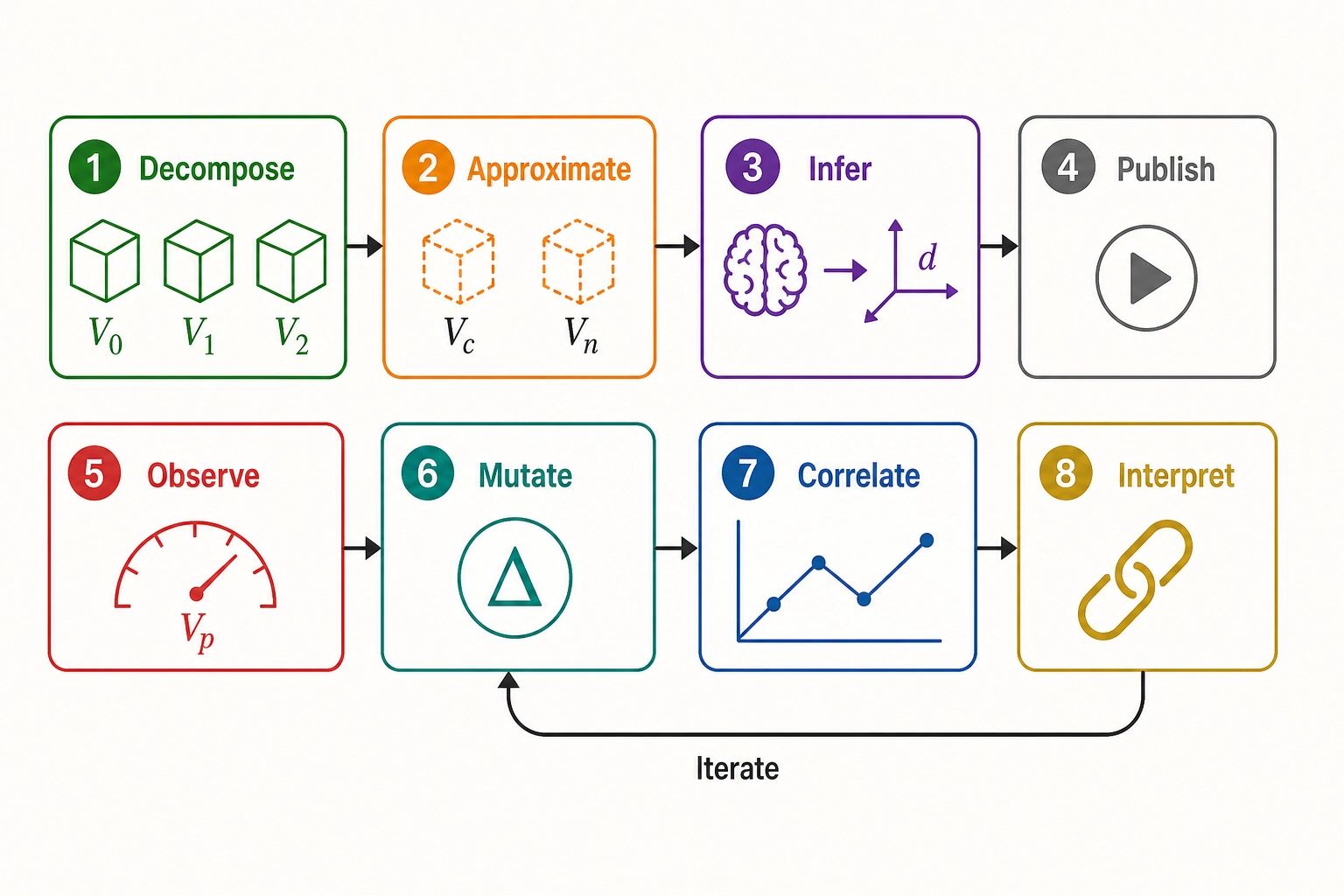
The 8-step pipeline in summary:
| Step # | Name | Input | Output | Vector(s) Involved |
|---|---|---|---|---|
| 1 | Decompose | Content file (pixels, audio, metadata) | Deterministic physical measurements | V₀, V₁, V₂ |
| 2 | Approximate | Content file | Cognitive labels and predicted cortical activation | Vc, Vₙ |
| 3 | Infer | Vₙ activation pattern + dimension architecture | Experiential-dimension engagement estimates | Vₙ mapped to Chapter 4 dimensions |
| 4 | Publish | Final content file | Published content under controlled conditions | None (operational step) |
| 5 | Observe | Published content + audience | Platform metrics and self-report | Vₚ |
| 6 | Mutate | Reference content + mutation operator | Variant content with measured V-delta | V₀ through Vₙ (layer depends on operator) |
| 7 | Correlate | Reference Vₚ + Variant Vₚ + V-delta | Effect estimates with confidence intervals | Vₚ, V-delta |
| 8 | Interpret | Effect estimates + Vₙ predictions + Vc-Vₙ consistency | Mechanistic interpretation with evidential labels | All vectors |
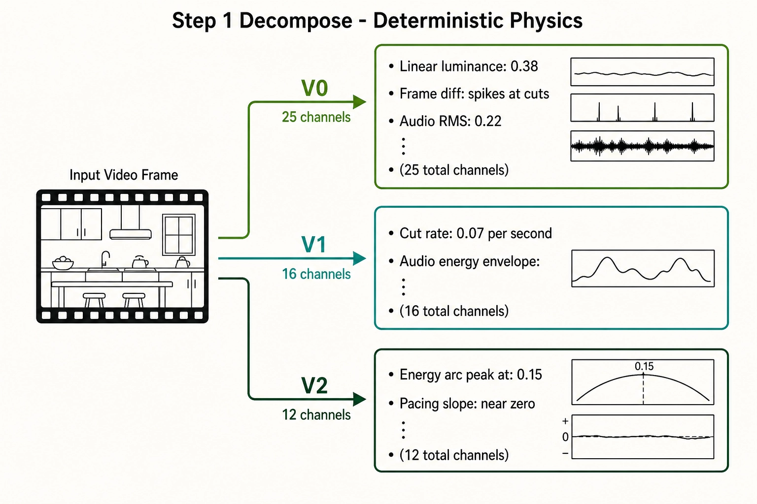
Step 1: Decompose - V₀, V₁, V₂
The content file enters the V₀ pipeline. Twenty-five channels are extracted using physics and arithmetic only. Linear luminance is computed per frame after removing the sRGB gamma curve: the kitchen scenes average 0.38, the overhead cooking shot averages 0.31 (the countertop is darker than the face-lit setup). Frame-to-frame luminance difference (v0.pixel.diff_l1) spikes at two points: the cut from face-to-camera to overhead (diff_l1 = 0.14, well above the cut-detection threshold of 0.08 as specified by v1 calibration values locked in Chapter 10) and the cut from overhead back to face-to-camera (diff_l1 = 0.11). Audio RMS energy averages 0.22 across the file, with a dip during the overhead segment where the music continues but voiceover pauses.
V₁ derives 16 channels from V₀ over three standard time windows (0.5-second short, 5-second medium, full-file). The pacing channel v1.pacing.diff_threshold_crossings reports 2 cuts in 28 seconds - a cut rate of approximately 0.07 cuts per second at the full-file scale, or about one cut every 14 seconds. The audio energy envelope (v1.energy.audio_rms_envelope) shows a three-segment contour: moderate energy during the face-to-camera opener, lower energy during the overhead, and a brief rise at the close.
V₂ derives twelve channels from V₁ across the file. The energy arc peak position (v2.shape.energy_argmax_fraction) is at approximately 0.15: the energy peaks early, in the first face-to-camera segment. The pacing slope (v2.derivative.pacing_slope) is effectively zero - with only two cuts, there is no acceleration or deceleration to measure.
All of these values are deterministic, reproducible, and free of perceptual models. Any system analyzing the same file produces identical numbers.

Step 2: Approximate - Vc, Vₙ
Vc runs the vision-language model (Gemini 2.5 Pro, temperature 0.0) directly on the content file. Vc spans 32 dimensions across 9 categories. It reports: vc_face_present = true on approximately 64% of frames (the face-to-camera segments), vc_face_count = 1, vc_expression_primary = happy (she is smiling throughout the direct-to-camera portions), vc_scene_setting = indoor_domestic, vc_objects_present includes cooking utensils and ingredients, vc_narrative_arc_position = setup → demonstration → resolution across the three segments. The predicted viewer emotion (vc_predicted_viewer_emotion_primary) is warmth_or_comfort: the model’s cognitive-level prediction about what the typical viewer would feel, not a measurement of what any viewer actually feels.
Vₙ runs TRIBE v2 on the same content file - no scanner, no subjects, just the file. The predicted cortical activation pattern across 360 Glasser areas at 1 Hz (one prediction per second) shows: strong fusiform face area (FFA - the cortical region with dedicated neural machinery for face processing) activation during the face-to-camera segments, dropping during the overhead shot and returning at the close. Primary auditory cortex (A1 - the cortical region that processes basic auditory features including pitch, rhythm, and temporal patterns) shows sustained activation throughout, tracking the continuous background music and voiceover. The default mode network (DMN - the cortical regions active when a person is relating what they see to their own life, imagining what might happen next, or reflecting inward) shows moderate activation, consistent with a video that invites personal identification (“I could make this at home”).
The Vc-Vₙ consistency check (Chapter 5 Section 8) runs. Vc says face is present; Vₙ predicts strong FFA activation. Agreement. Vc says spoken language is present; Vₙ predicts Broca’s area (the inferior frontal cortical region for speech production and processing) activation. Agreement. Confidence in both rises.
Step 3: Infer
From Vₙ’s predicted activation pattern and the dimension architecture in Chapter 4, the framework infers which aspects of the viewer’s perception and emotion are likely engaged. FFA activation maps to the social-cognition dimension at Resolution Level 2: the viewer’s brain is processing social information (a human face, expressions, identity). A1 activation maps to the auditory dimension: the viewer’s brain is processing the music and voice. DMN activation maps to the self-reference dimension: the viewer is likely relating the content to their own life.
Khozai can identify the processing dimensions involved (social, auditory, self-referential), estimate their activation magnitude (FFA activation is strong during face segments, moderate during the overhead), and assess their independence (FFA and A1 show distinct temporal profiles - they are not tracking the same stimulus feature). What remains opaque is the subjective quality of any of it. The warm familiarity of watching someone cook, the specific quality of hearing a particular voice: that is Scope B of Experience Space, structurally opaque, accessible only through what viewers report.
Step 4: Publish
The video is published under standard conditions: same account, no paid promotion, platform auto-mutation tools disabled (Chapter 7 Section 5).
Step 5: Observe - Vₚ and self-report
After publication, Vₚ collects twenty-two platform metrics at defined intervals. The key outcomes: average view duration is 18.4 seconds (65.7% of the 28-second file), completion rate is 0.41 (41% of viewers watched to the end), engagement rate is 4.2%, share rate is 0.3%.
The self-report extraction pipeline (Chapter 6) processes the comment section. Three outputs are produced. Scope A dimension estimates identify activation of the self-referential and affective dimensions (“this reminds me of my mom’s cooking,” “I need to try this”). Scope B qualitative summaries capture what viewers reported experiencing in their own words: warmth, nostalgia, practical interest. Construct-confirmation labels tag the “reminds me of my mom” comments as confirming a Self + Memory + Affect pattern - the signature of nostalgia as a psychological construct mapped across experiential dimensions (Chapter 4 Section 5).
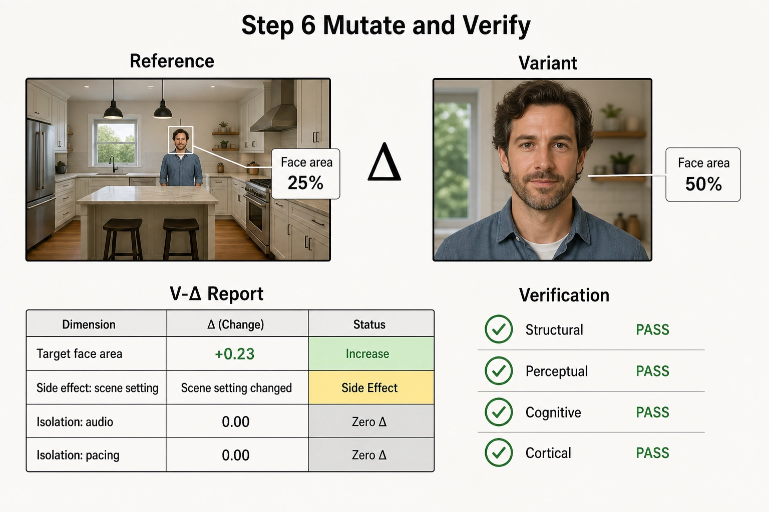
Step 6: Mutate - V-delta
Now the mutation engine enters. The platform’s second-by-second retention data shows a drop at the transition from face-to-camera to overhead. Hypothesis: increasing the fraction of the frame occupied by the face would increase retention.
The mutation engine applies op_face_area (crop_to_face method) to increase the face-area fraction from approximately 25% to approximately 50%. The four-layer verification pipeline confirms: structural verification passes, perceptual verification confirms the face-area fraction shifted to 0.48 (within the +/- 5% tolerance), cognitive verification confirms vc_face_present is still true and vc_face_count is unchanged, and cortical verification confirms an increase in predicted FFA activation.
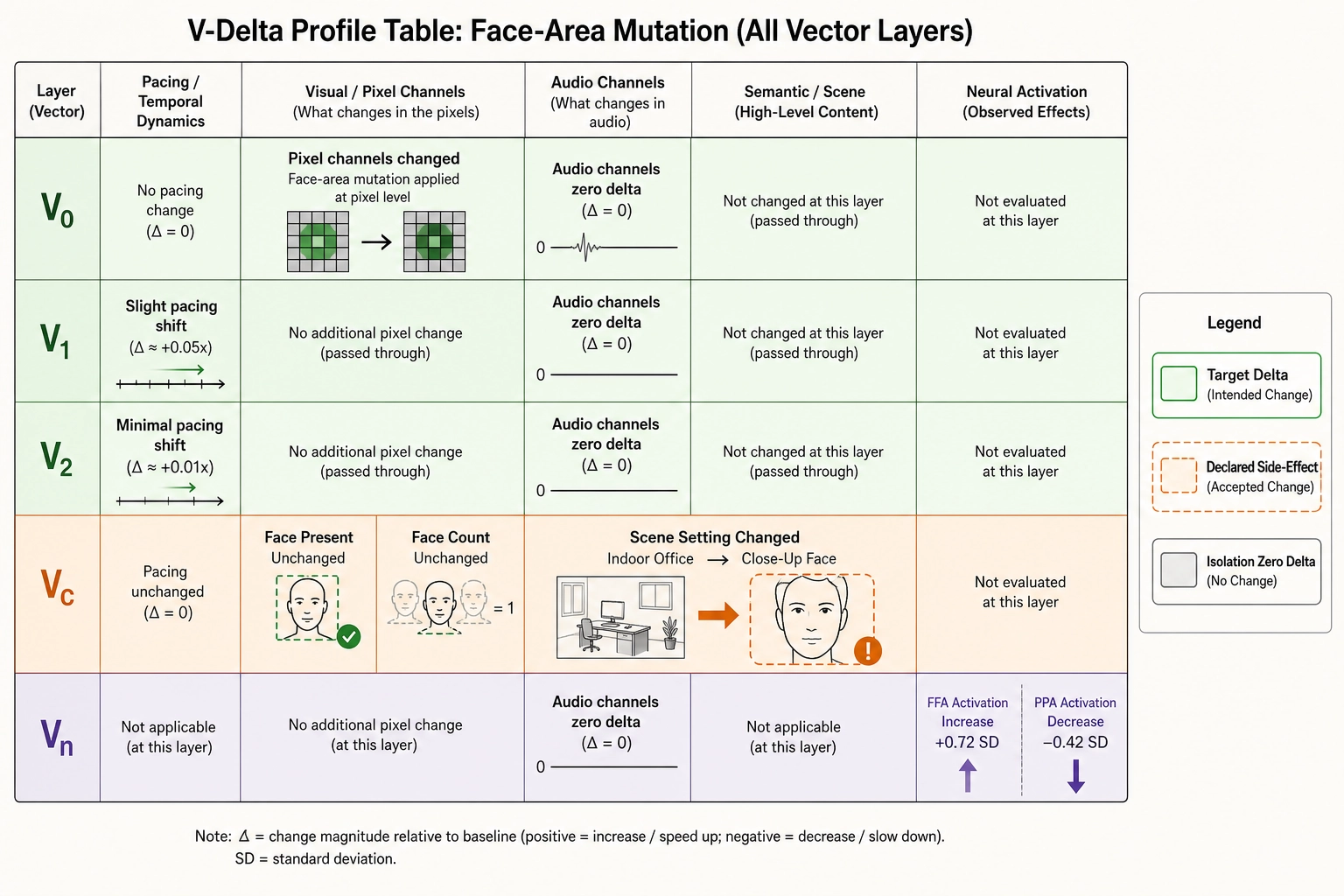
V-delta is computed at every layer. The targeted V-delta: face-area fraction +0.23 (from 0.25 to 0.48). The declared side-effect: vc_scene_setting shifted from indoor_domestic to close_up_face on the face-to-camera frames - the crop removed the kitchen context. This is an expected side-effect of the crop method, logged as declared. Isolation V-delta on audio channels: zero (the operator did not touch audio). Isolation V-delta on pacing: zero (the cut structure is unchanged).
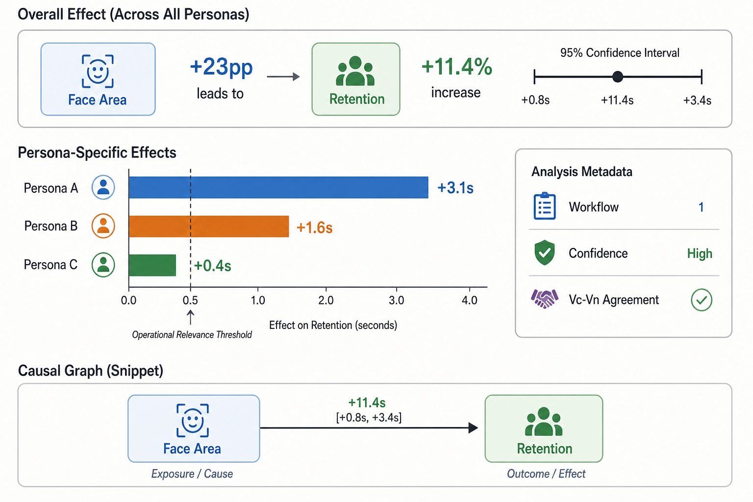
Step 7: Correlate
Both versions - reference and variant - are published under identical conditions (same account, same budget, same platform split-test randomization). Vₚ data are collected. The correlation engine (Chapter 8, workflow 1 - controlled mutation) estimates the effect: face area +23 percentage points → average view duration +2.1 seconds (from 18.4 to 20.5 seconds), a +11.4% relative increase. The 95% confidence interval is [+0.8s, +3.4s]. The confidence interval excludes zero. The effect exceeds the Vₚ operational-relevance threshold of 0.5 seconds, a v1 calibration value locked in Chapter 10 - it is both statistically detectable and operationally meaningful.
The effect is computed per persona. Persona A (high-engagement viewers who comment and share) shows +3.1 seconds. Persona B (passive viewers who watch but rarely interact) shows +1.6 seconds. Persona C (browsers who typically drop off within the first 5 seconds) shows +0.4 seconds - below the 0.5-second operational-relevance threshold. The persona-level heterogeneity reveals that the face-area effect is concentrated among viewers who are already somewhat engaged.
Step 8: Interpret
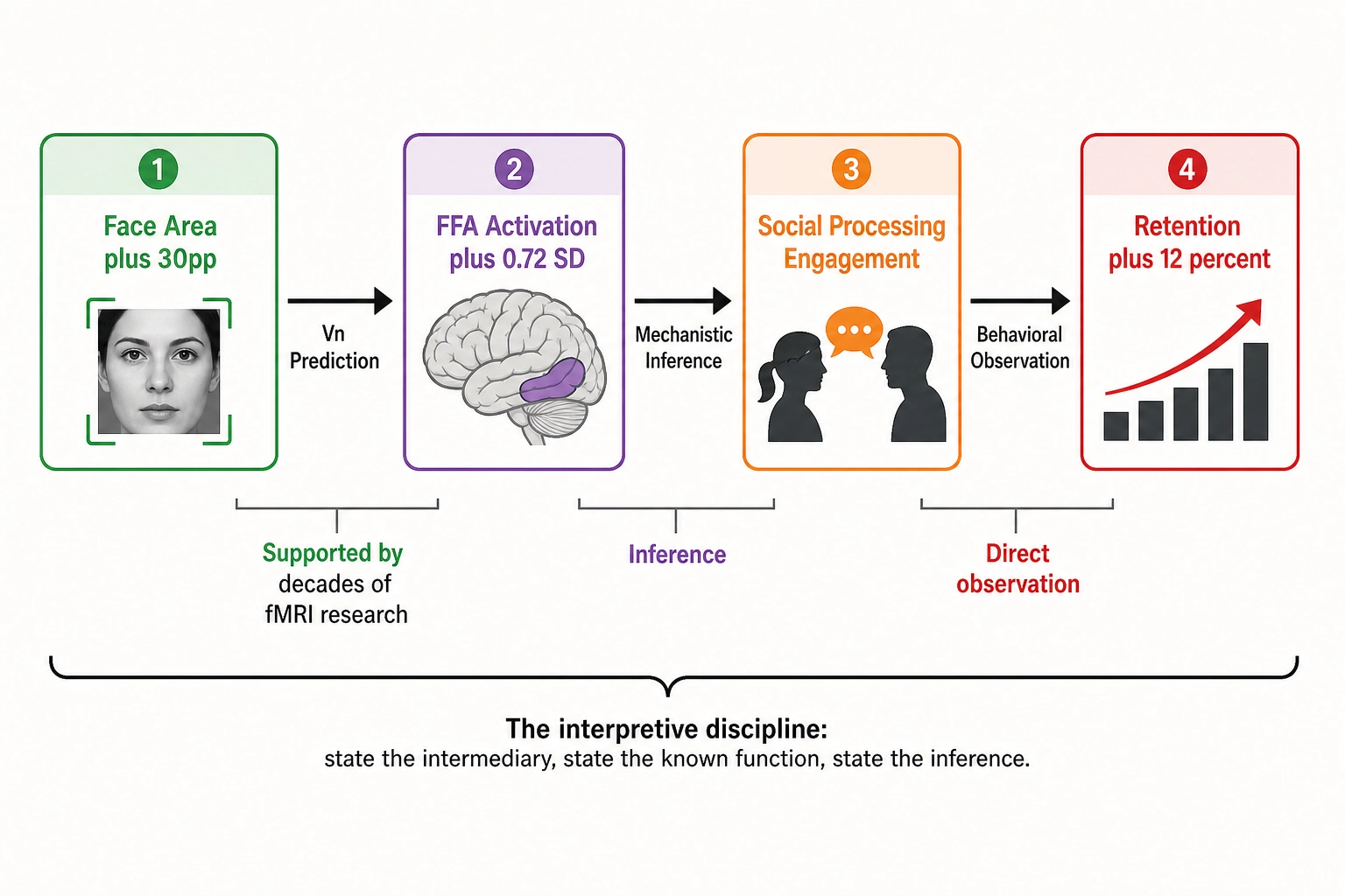
The interpretive step adds the cortical intermediary from Vₙ. The Vc-Vₙ consistency check confirms: Vc detected a larger face, Vₙ predicted stronger FFA activation. The interpretation becomes: larger face → stronger predicted FFA activation → stronger social-processing engagement → continued watching. Each link has a different evidential status. The first is supported by the Vₙ prediction and by published research showing that lower-level stimulus features such as face size strongly influence FFA responses (Yue, Vessel, & Biederman, 2011 [5]). The second - that stronger FFA activation produces stronger social-processing engagement sufficient to drive continued watching - is a mechanistic inference, not an established causal finding; no published study has directly demonstrated that FFA activation magnitude predicts viewing retention. Whether such a study would find a positive result is unknown - the absence of evidence is not evidence of absence, but neither is it evidence of the mechanism the chain assumes. The third is the behavioral observation. The chain is plausible, not proven - Bet 2 supplies the first link, and the framework’s accumulated evidence either strengthens or weakens it over time.
This is the full pipeline: decompose, approximate, infer, publish, observe, mutate, correlate, interpret. Every step is traceable, every number is auditable, every inference is labeled as an inference. What follows are three worked examples that walk specific mutations through this chain.
2. Worked Example 1: Face-Area Mutation
section 1 walked the face-area mutation through all eight pipeline steps on the cooking video. This worked example uses a different video to isolate what the face-area operator reveals about the framework’s layer-crossing architecture, focusing on the V-delta profile, calibration mechanics, and the PPA trade-off that the end-to-end walkthrough introduced but did not examine in detail.
The mutation
Reference: a 22-second vertical video of a person speaking to camera. Face-area fraction is 0.22 (22% of the frame is occupied by the face). The background is a blurred office setting.
Variant: op_face_area (crop_to_face method, deterministic, tier 1) applied with target_face_area_fraction = 0.52. The crop centers on the face bounding box and scales to the project resolution. The resulting face-area fraction is 0.50 - within the +/- 5% tolerance declared by the operator.
V-delta profile
V₀: All pixel-domain channels change (new spatial content). Audio channels: zero delta (untouched). Container metadata: zero delta (same duration, same frame rate).
V₁: Pixel-derived pacing channels shift slightly (the inter-frame differences change because different spatial content is being compared). Audio-derived channels: zero delta. The cut rate is unchanged - same number of cuts, same timing.
V₂: Downstream of V₁; minimal shift.
Vc: vc_face_present unchanged (true). vc_face_count unchanged (1). vc_expression_primary unchanged (the same face with the same expression). vc_scene_setting changed - from indoor_office to close_up_face on the affected frames. This is the declared side-effect of the crop method: the background context is lost.
Vₙ: Predicted FFA activation increases. The increase is 0.72 standard deviations above the reference-corpus mean for FFA - above the Vₙ activation-shift threshold of 0.5 standard deviations, a v1 calibration value locked in Chapter 10. This registers as a meaningful cortical shift, not noise. Predicted activation in parahippocampal place area (PPA - the cortical region involved in scene and place processing) decreases - consistent with the loss of background scene context from the crop.
Calibration check
The v1 calibration values (locked in Chapter 10) consumed here:
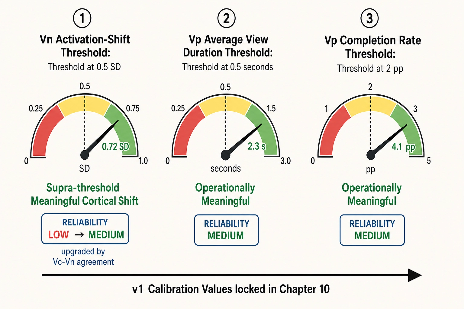
- Vₙ activation-shift threshold: 0.5 SD change in parcel-level predicted activation. The FFA shift of 0.72 SD exceeds this. Classification: supra-threshold, meaningful cortical shift.
- Vₚ average-view-duration operational-relevance threshold: 0.5 seconds. The observed effect is +2.3 seconds. Classification: operationally meaningful.
- Vₚ completion-rate operational-relevance threshold: 2 percentage points. The observed effect is +4.1 pp (completion rate from 0.38 to 0.42). Classification: operationally meaningful.
Tag reliability for the Vₙ threshold: LOW (derived from a small reference corpus, per Chapter 10). Tag reliability for the Vₚ thresholds: MEDIUM (normative operational judgments). The Vc-Vₙ consistency check upgrades the effective tag reliability by one level per the operational rule Chapter 10 will specify: the FFA shift’s tag reliability goes from LOW to MEDIUM because Vc and Vₙ agreed on the face-area change.
The inference chain
The interpretive logic follows the same path as Section 1’s cooking-video example: larger face → stronger predicted FFA activation → plausibly stronger social-processing engagement → continued watching (see Section 1, Step 8 for the full chain and its evidential labels; the FFA-to-retention behavioral link remains an inference, not an established causal finding). What this second video adds is the PPA trade-off and the calibration mechanics.
- Content property change (V₀/Vc): Face-area fraction increased from 0.22 to 0.50.
- Predicted cortical consequence (Vₙ): FFA activation increased by 0.72 SD. PPA activation decreased (scene context lost to the crop).
- Behavioral outcome (Vₚ): Average view duration +2.3 seconds; completion rate +4.1 pp. Per-persona: strongest for personas A and B, negligible for persona C.
- Trade-off: Social processing outweighed scene processing for this content - but the PPA decrease means the crop method is not cost-free. Content where scene context carries the engagement signal (e.g., travel or architecture videos) could show the opposite result.
What this example shows
Three architectural features. First, the Vc-targeted, V₀-touching classification: the mutation requires cognitive recognition (finding the face) and produces physical change (cropping pixels). Neither “V₀ mutation” nor “Vc mutation” is accurate alone. Second, the declared side-effect: the scene-composition change is not a failure of isolation - it is a known, measured consequence of the crop method. Third, the v1 calibration values (locked in Chapter 10) transform raw numbers into interpretive categories: a 0.72 SD cortical shift is “meaningful” because the threshold says so; a +2.3-second behavioral shift is “operationally relevant” because the threshold says so. Without the calibration values, the numbers are just numbers.
3. Worked Example 2: Audio-Tempo Mutation
The second example targets a different modality - audio - and exposes the confidence differential between cortical and subcortical predictions.
The operator
op_time_stretch changes the playback speed of a segment or scene using a phase-vocoder algorithm that preserves pitch while changing duration. It is a V₀-targeted operator (tier 1, deterministic) that shifts audio and visual temporal structure simultaneously.
The mutation
Reference: a 30-second vertical video with background music at approximately 95 beats per minute (BPM). The dominant autocorrelation lag in V₁ (v1.autocorr.audio_rms_peak_lag) is 0.632 seconds, corresponding to the 95 BPM pulse. The video has moderate pacing - 3 cuts in 30 seconds (0.1 cuts per second).
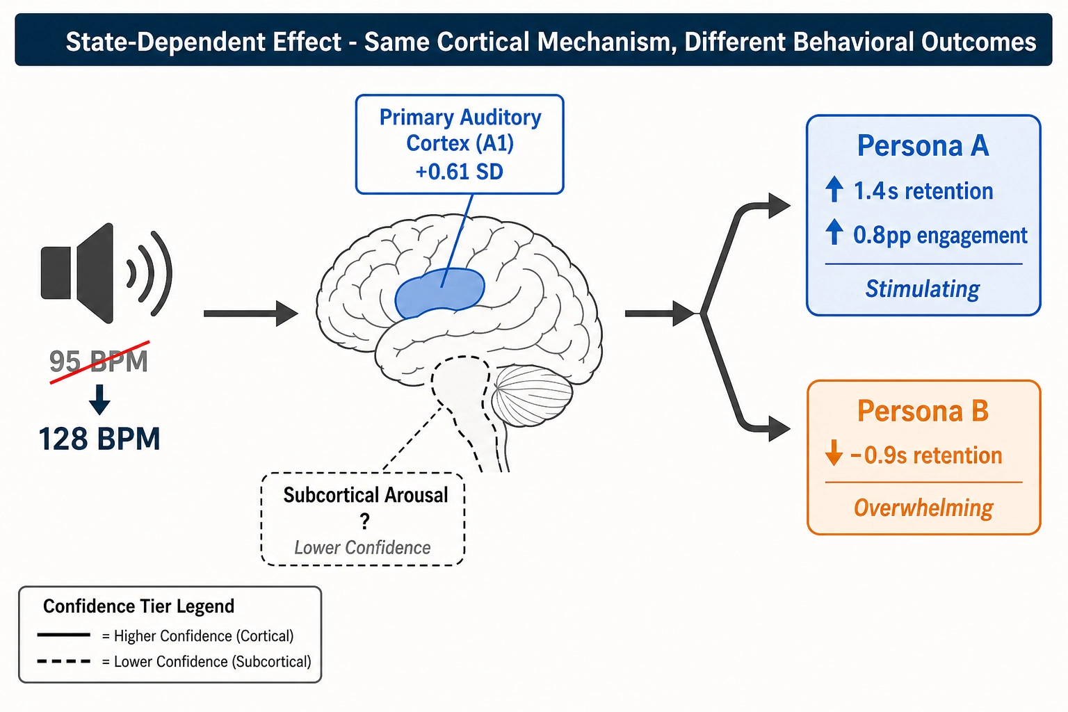
Variant: op_time_stretch applied with rate = 1.35 to the audio track only (the visual timeline is unchanged). The audio tempo shifts from approximately 95 BPM to approximately 128 BPM. The dominant autocorrelation lag shifts from 0.632 seconds to 0.469 seconds - a change of 0.163 seconds.
V-delta profile
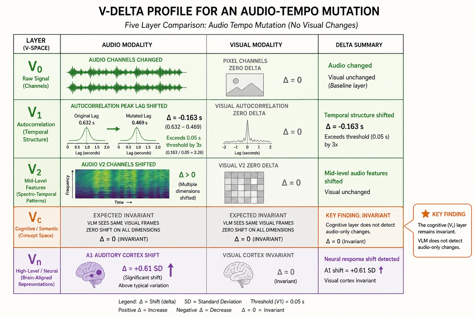
V₀: Audio channels change: v0.audio.waveform_mono and v0.audio.waveform_stereo are time-stretched. v0.audio.rms is approximately invariant (time-stretch preserves amplitude envelope shape). v0.audio.spectral_centroid shifts slightly (phase-vocoder artifacts). v0.audio.zero_crossing_rate changes (the waveform shape changes). Pixel channels: zero delta (the visual timeline is unchanged).
V₁: v1.autocorr.audio_rms_peak_lag shifts from 0.632 to 0.469 seconds - a V-delta of -0.163 seconds. This exceeds the calibration threshold of 0.05 seconds (a v1 calibration value locked in Chapter 10) by a factor of more than three. Classification: supra-JND, the tempo change is well above the threshold where it would be perceived.
V₂: Audio-derived V₂ channels shift (the temporal structure of the audio is different). Visual-derived V₂ channels: zero delta.
Vc: Expected invariant: the vision-language model receives the same visual frames, and the tempo change in background music does not change what the model recognizes. Vc reports no shift on any dimension. This is the expected behavior for a V₀ audio mutation that does not affect speech intelligibility.
Vₙ: Predicted shift in primary auditory cortex (A1) activation pattern: the cortical encoding model receives a different audio stimulus. The shift is 0.61 SD in A1, above the 0.5 SD activation-shift threshold. Adjacent auditory association areas show smaller shifts. Visual cortex areas: invariant (the visual stimulus is unchanged).
Calibration check
v1.autocorr.audio_rms_peak_lagthreshold: 0.05 seconds (v1 calibration value, locked in Chapter 10). The shift of 0.163 seconds is supra-JND. Tag reliability: LOW (derived, not directly measured).- Vₙ activation-shift threshold: 0.5 SD. The A1 shift of 0.61 SD exceeds this. Tag reliability: LOW, elevated to MEDIUM by Vc-Vₙ consistency (Vc reports no face or speech change, and Vₙ shows the shift is localized to auditory cortex - the two are consistent in showing an audio-only effect).
- Vₚ thresholds: average view duration threshold 0.5 seconds; engagement rate threshold 0.5 pp.
The behavioral outcome
The Vₚ outcome varies by persona - and this is where the example becomes instructive.
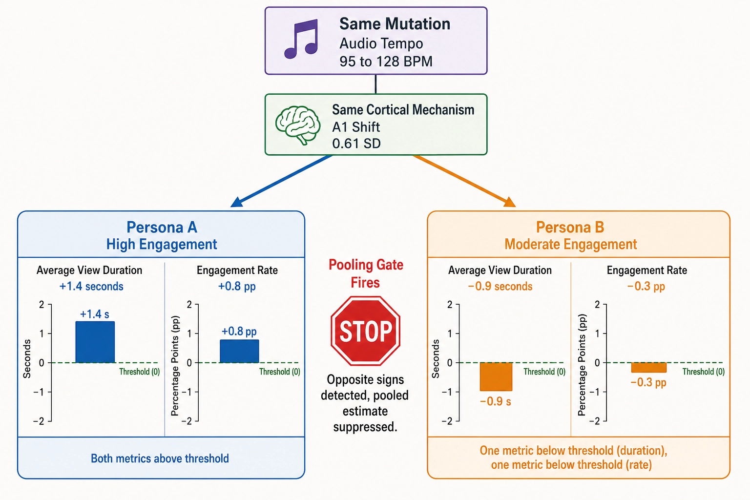
Persona A (high-engagement cluster, higher engagement baseline): average view duration +1.4 seconds, engagement rate +0.8 pp. Both above operational-relevance thresholds.
Persona B (moderate-engagement cluster, moderate engagement baseline): average view duration -0.9 seconds, engagement rate -0.3 pp. The duration effect exceeds the 0.5-second threshold but in the negative direction.
The pooling gate from Chapter 8 Section 4 fires: the per-persona effects have opposite signs. The pooled estimate is suppressed and replaced with a per-persona breakdown. The same audio-tempo mutation increased engagement for one group and decreased it for another.
The inference chain - and its structural limitation
- Content property change (V₀): Audio tempo increased from 95 BPM to 128 BPM.
- Detected temporal pattern change (V₁): Dominant autocorrelation lag shifted by -0.163 seconds, supra-JND.
- Predicted cortical consequence (Vₙ): A1 activation pattern shifted by 0.61 SD. The cortical encoding model predicts a change in how auditory cortex processes the faster tempo.
- Inferred experiential engagement: Cortical-side correlates of arousal modulation. The auditory cortex shift is consistent with a change in the brain’s processing of rhythmic stimulation.
Here the chain encounters a confidence differential. Arousal itself - the global activation level that determines how alert and responsive a person is - is regulated by subcortical structures: the brainstem’s reticular activating system and the locus coeruleus (a brainstem structure that modulates alertness through norepinephrine release). Khozai predicts activation in these subcortical structures with lower confidence than cortical predictions due to fMRI SNR limitations. The predictions are included because arousal regulation is among the most relevant signals for content engagement. Cortical-side correlates of arousal modulation - auditory cortex activation patterns, salience network engagement - enter at higher confidence.
The interpretation is therefore: faster audio tempo → altered A1 activation pattern → cortical-side correlates of arousal modulation (higher confidence) and predicted subcortical arousal regulation (lower confidence) → different behavioral outcomes depending on persona. The language distinguishes confidence tiers: “cortical-side correlates of arousal modulation” for the higher-confidence claims, “predicted subcortical arousal regulation” for the lower-confidence claims. This is not a failure of the framework. It is the confidence-tiered design working as intended - subcortical predictions contribute signal, and the confidence differential is stated honestly. The cortical correlates carry the stronger signal; the subcortical predictions add coverage of the arousal pathway at a cost of lower certainty.
What this example shows
Three things. First, a V₀ audio mutation can produce supra-JND temporal pattern changes (V₁) and meaningful cortical shifts (Vₙ) while leaving the cognitive layer (Vc) invariant: the VLM does not notice the tempo change. Second, the per-persona heterogeneity is not noise - it is a finding. The same cortical mechanism produces opposing behavioral outcomes for different viewer groups, a concrete instance of Tool 11’s state-dependence axis (Chapter 8 Section 7). Third, the confidence differential between cortical and subcortical predictions (described above) means the inference chain carries two tiers of certainty, and the framework’s language must distinguish them.
4. Worked Example 3: Cut-Rate Mutation
The third example targets visual pacing - the temporal structure of the video itself - and tests the framework’s ability to measure attentional-demand modulation.
The operator
op_retime changes the duration of specific scenes, scaling their segments proportionally and time-stretching their audio to maintain synchronization. It is a V₁-targeted operator (tier 1, deterministic). By shortening scenes - making each scene occupy less time - the effective cut rate increases without changing any scene’s internal spatial content.
The mutation
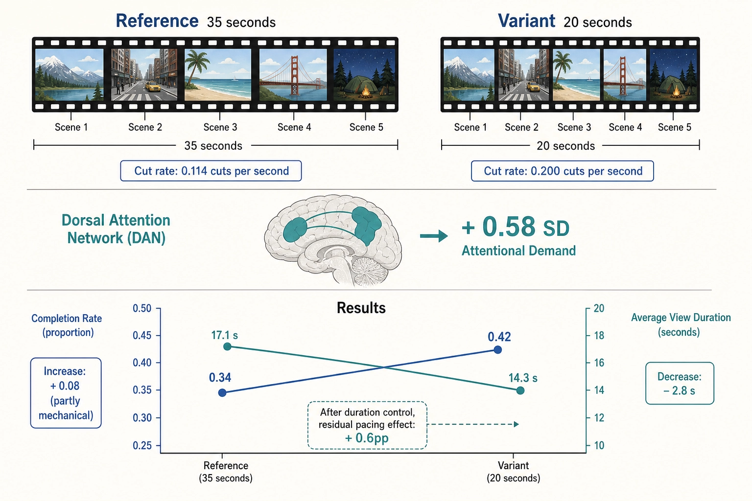
Reference: a 35-second vertical video with 5 scenes of varying length (8s, 10s, 7s, 6s, 4s). The cut rate (v1.pacing.diff_threshold_crossings at the full-file window) is 4 cuts in 35 seconds = 0.114 cuts per second. V₀’s frame-to-frame luminance difference spikes above the 0.08 threshold at each scene boundary.
Variant: op_retime applied to shorten each scene by a uniform factor, producing a 20-second video with the same 5 scenes (4.6s, 5.7s, 4.0s, 3.4s, 2.3s). The cut rate is now 4 cuts in 20 seconds = 0.200 cuts per second. Each scene’s internal content is preserved - the same frames appear in the same order - but the playback speed is 1.75x within each scene. Audio is time-stretched (pitch preserved).
V-delta profile
V₀: v0.meta.duration changed from 35 to 20 seconds. Audio channels change (time-stretched waveform). Per-frame pixel content within each scene is preserved (same spatial content, different temporal spacing). Frame-difference channels (v0.pixel.diff_l1) shift because the inter-frame time interval is different.
V₁: v1.pacing.diff_threshold_crossings shifted from 0.114 to 0.200 cuts per second - a V-delta of +0.086 cuts per second. Against the calibration threshold of 0.3 cuts per second (v1 calibration value, locked in Chapter 10), this is sub-JND - below the published threshold for when viewers reliably perceive a pacing difference as a distinct change in rhythm. However, that calibration value also carries LOW tag reliability (derived, not directly measured), so the sub-JND classification is tentative.
The audio-derived V₁ channels shift more dramatically. The time-stretch changes the audio energy envelope, onset rate, and autocorrelation structure. v1.energy.audio_rms_window_var increases (the faster tempo compresses the energy dynamics into a shorter window, increasing the variance per unit time).
V₂: v2.derivative.pacing_slope is still effectively zero (the uniform retiming preserves the relative scene proportions). But v2.shape.energy_arc_peak_position shifts - the energy arc is compressed into a shorter file, and the peak position (as a fraction of the file) may move.
Vc: Expected invariant for moderate retiming. The per-frame visual content is unchanged, so the VLM recognizes the same objects, faces, and scenes. vc_narrative_arc_position may shift if the pacing change alters perceived narrative rhythm, but for a 1.75x speed-up, the model’s per-video assessment is likely stable.
Vₙ: The cortical encoding model receives a different temporal stimulus. Predicted visual processing load increases - V1 (primary visual cortex, not to be confused with the V₁ vector) and higher visual areas show increased activation density per unit time, because the same visual content is being processed at a faster rate. The dorsal attention network - the cortical network that controls voluntary attention allocation - shows a predicted increase in activation, consistent with greater attentional demand. Direct fMRI evidence isolating the dorsal attention network specifically for editing-pace variation remains limited; the attribution is based on the DAN’s established role in voluntary attention allocation (the attention researchers Maurizio Corbetta and Gordon Shulman, 2002 [8]) and EEG evidence of frontal attention-network engagement during film cuts (the neuroscientist Katrin Heimann and colleagues, 2017 [9]). High-density EEG data show that different editing techniques produce distinct neural signatures in attention-related cortical networks (Heimann et al., 2017 [9]), and attention allocation to Hollywood films tracks the evolution of editing rates across decades (the psychologist James Cutting and colleagues, 2010 [10]). The shift in dorsal attention network activation is 0.58 SD, above the 0.5 SD threshold.
Calibration check
v1.pacing.diff_threshold_crossingsthreshold: 0.3 cuts per second (v1 calibration value, locked in Chapter 10). The shift of 0.086 is sub-JND. But tag reliability is LOW. The cut-rate change, while below the published pacing-perception threshold, is accompanied by a substantial duration change (35s to 20s) that viewers will certainly notice. The calibration value for pacing perception applies to pacing within a video of constant length - not to the compound change of shorter video + faster scenes.- Vₙ activation-shift threshold: 0.5 SD. The dorsal attention network shift of 0.58 SD exceeds this.
- Vₚ thresholds: completion rate threshold 2 pp; average view duration threshold 0.5 seconds.
The behavioral outcome
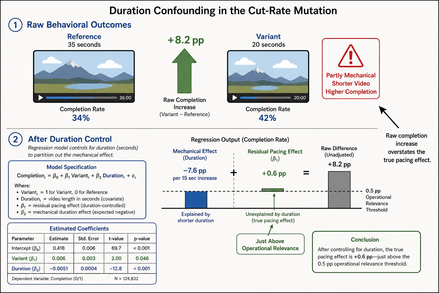
Completion rate increases by 8.2 pp (from 0.34 to 0.42) - not because the content is more engaging, but partly because the video is shorter (20 seconds versus 35 seconds, so completing it requires less commitment). Average view duration decreases by 2.8 seconds (from 17.1 to 14.3 seconds) - viewers watched a smaller absolute amount, but a larger fraction of the shorter video.
This is a case where the Vₚ outcome requires careful interpretation. The completion-rate increase is partly mechanical (shorter video → higher completion) and partly behavioral (faster pacing may maintain attention more effectively). The average-view-duration decrease is also partly mechanical (shorter video → shorter possible duration). The correlation engine must control for content duration as a covariate - which it does, using v0.meta.duration as a standard covariate in the regression (Chapter 8 Section 2). After controlling for duration, the residual pacing effect on engagement rate is +0.6 pp - just above the 0.5 pp operational-relevance threshold.
The inference chain
-
Content property change (V₀/V₁): Cut rate increased from 0.114 to 0.200 cuts per second. File duration decreased from 35 to 20 seconds. Per-scene playback speed increased to 1.75x.
-
Predicted cortical consequence (Vₙ): Dorsal attention network activation increased by 0.58 SD. Visual processing load increased.
-
Inferred experiential engagement: Attentional-demand modulation. The viewer’s voluntary attention system is working harder to keep up with the faster-paced content. Whether this is experienced as stimulating or overwhelming depends on the viewer.
-
Behavioral outcome (Vₚ): Higher completion rate (partly mechanical), lower absolute duration (mechanical), and a small positive residual pacing effect on engagement rate after controlling for duration.
-
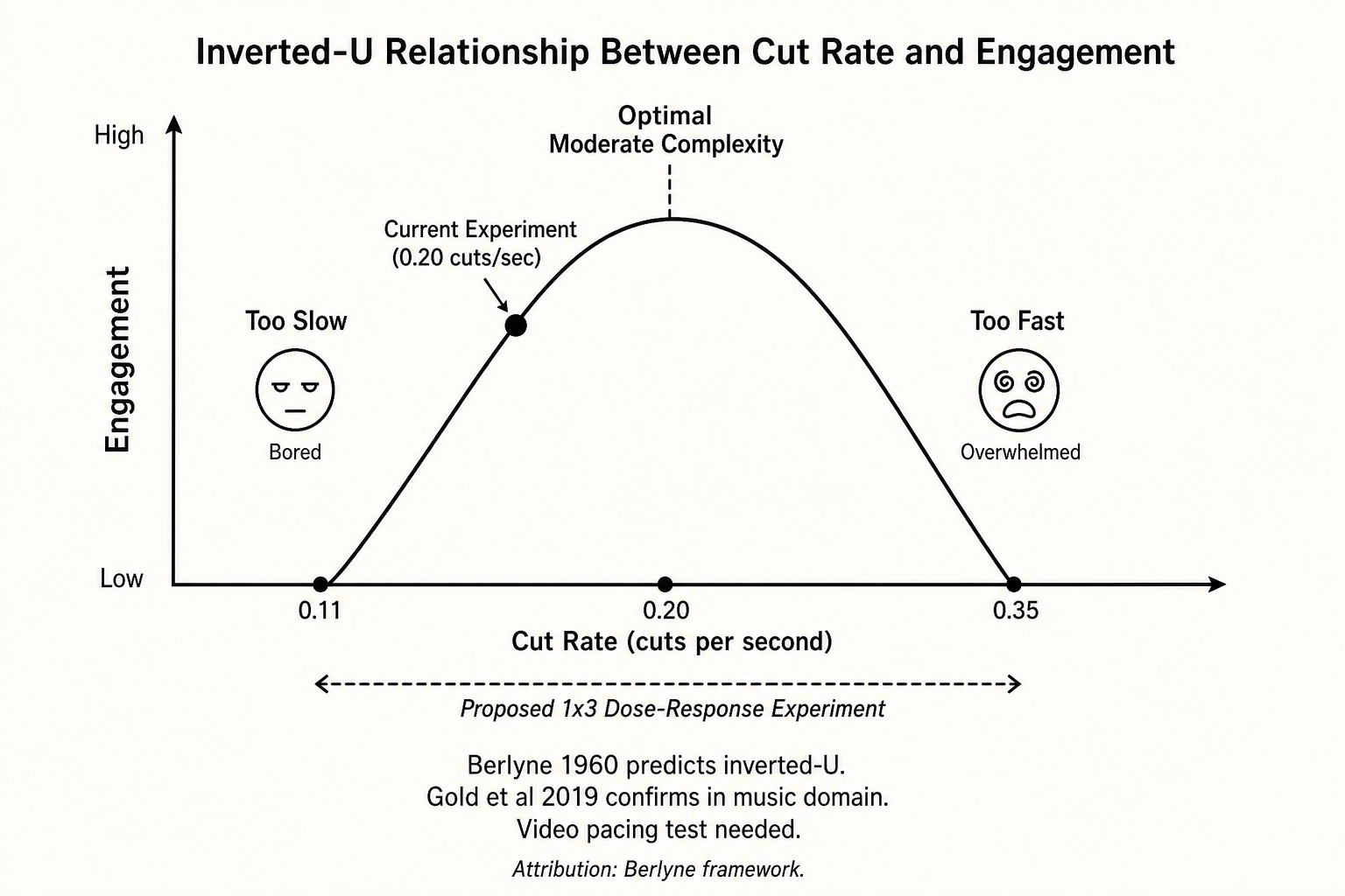
Interpretation: Faster pacing → higher predicted visual processing load → increased attentional demand → varied behavioral consequences. The inverted-U relationship theorized by Berlyne (1960) - that moderate complexity produces the strongest positive response - predicts that further increases in cut rate would eventually produce negative effects. Supporting evidence from a related perceptual domain: the neuroscientist Benjamin Gold and colleagues (2019 [11]) demonstrated significant quadratic (inverted-U) effects of information content on liking in music, where moderate predictability produced peak pleasure while both high predictability and high surprise reduced it. Though measured in music rather than video pacing, the finding is consistent with Berlyne’s framework applied to temporal information rate. A dose-response experiment (1x3 design: 0.11, 0.20, and 0.35 cuts per second) would test this prediction in the visual pacing domain.
What this example shows
Three things. First, V₁ changes (pacing) can be sub-JND on the calibration table and still produce meaningful cortical and behavioral effects - because the calibration threshold has LOW reliability and because the pacing change was confounded with a duration change. This is the calibration system working as designed: the LOW tag signals that the sub-JND classification should be held lightly. Second, behavioral outcomes require covariate control - the raw completion-rate increase is partly a mechanical artifact of shorter duration, not a pure pacing effect. Third, the example motivates a dose-response follow-up - one of the experimental design escalations from Chapter 7 Section 5 - because the hypothesis of an inverted-U relationship cannot be tested with a single mutation magnitude.
5. Where the Chain Breaks
The three worked examples show the inference chain functioning as designed. But the chain does not always hold. This section applies Tool 8 (Feedback Loop Test) from Chapter 2 Section 6.8 to classify the types of breakage.
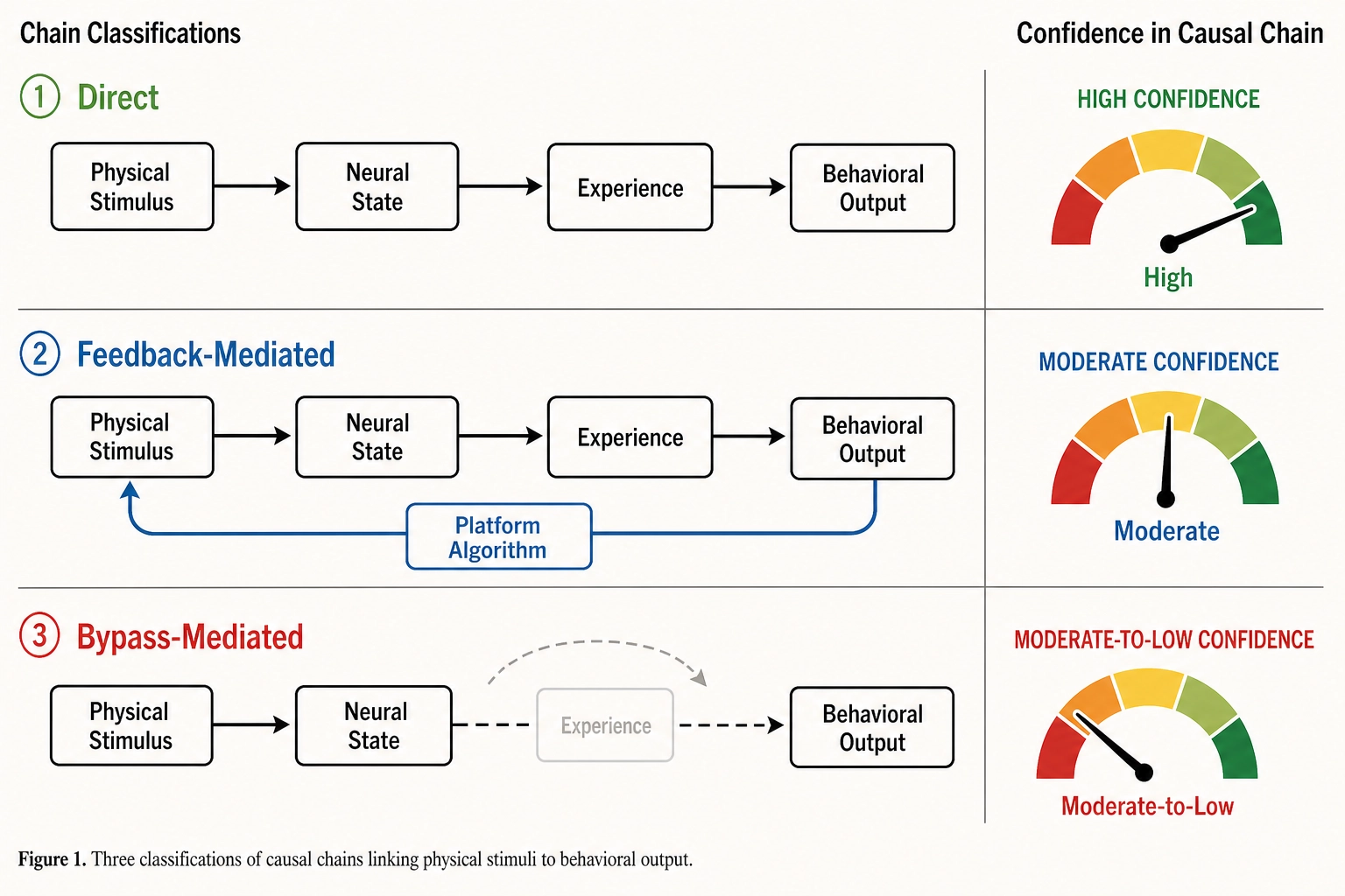
Tool 8’s procedure: given a correlation between a property in one space and a measurement in another, determine whether the pathway is direct, feedback-mediated, or bypass-mediated. Each classification has different implications for what the correlation means and how much causal confidence it supports.
The three chain-breakage classifications:
| Classification | Definition | Causal Confidence |
|---|---|---|
| Direct | X → Y through a single mapping traversal: Physical Stimulus → Neural State → Experience → Behavioral Output. Each link crosses one mapping. | High - bounded by operator isolation quality, statistical power, and Vₙ prediction accuracy (Bet 2). |
| Feedback-mediated | X → Y → Z → X → Y. The behavioral outcome changes the physical stimulus (e.g., platform algorithm serves new content), which re-enters the chain. The loop closes within the measurement window. | High for the direct component (single-session). Moderate for the feedback component (confounded by platform-specific algorithmic behavior). |
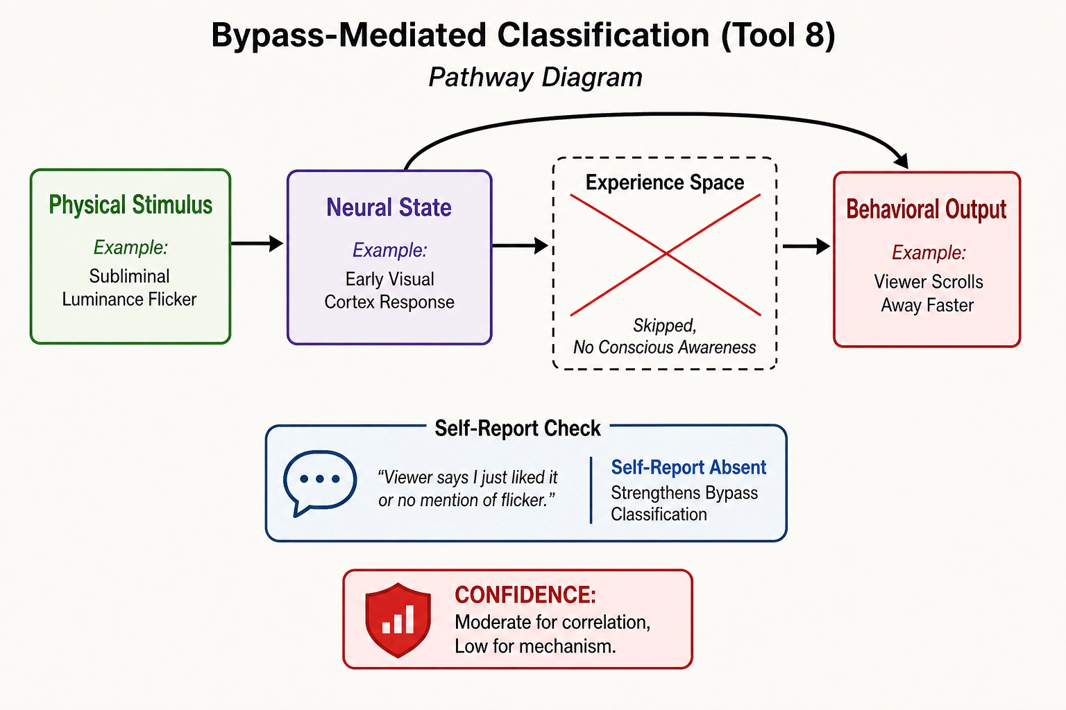
| Bypass-mediated | X → Neural State → Y without passing through Experience Space. The content property produces a neural response that directly drives behavioral output without conscious experience (e.g., subliminal processing, implicit arousal shifts). | Moderate for the property-to-outcome correlation. Low for the mechanistic interpretation (the experiential intermediary may not exist). |
Classification 1: Direct
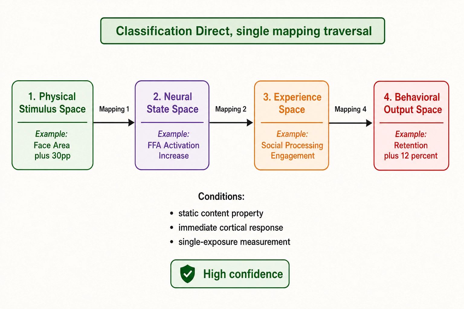
Definition: X → Y through a single mapping. A content property (Physical Stimulus Space or Neural State Space) maps to a behavioral outcome (Behavioral Output Space) through one traversal of the mapping chain: Physical Stimulus → Neural State (Mapping 1) → Experience (Mapping 2) → Behavioral Output (Mapping 4). Or, for Vₙ-level properties, Neural State → Experience → Behavioral Output.
Example from the worked examples: Face-area increase (Physical Stimulus Space) → FFA activation increase (Neural State Space, via Mapping 1) → stronger social processing (Experience Space, via Mapping 2) → continued watching (Behavioral Output Space, via Mapping 4). Each link crosses one mapping. The chain is direct.
When direct classification holds: When the content property is static (does not change during viewing), the cortical response is immediate (within the 1-2 second temporal resolution of Vₙ), and the behavioral outcome is measured after a single exposure. Most single-variable mutation experiments produce direct correlations because the mutation is applied once and the outcome is measured once.
Classification 2: Feedback-mediated
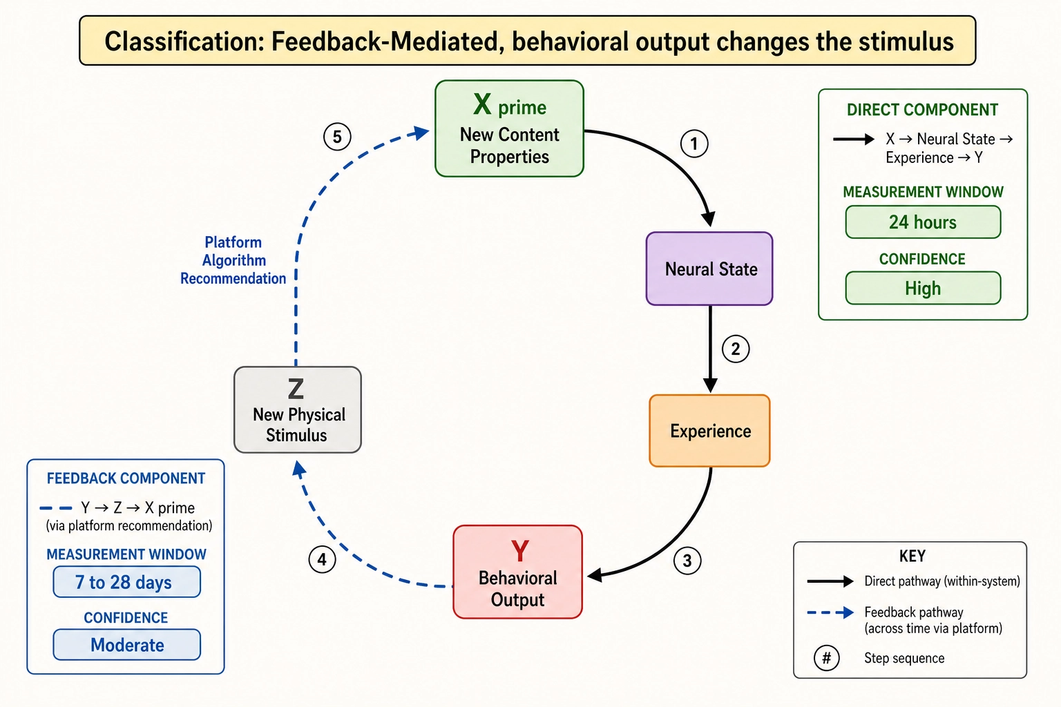
Definition: X → Y → Z → X → Y. The initial property produces a behavioral outcome, and that behavioral outcome changes the physical stimulus, which re-enters the chain and produces another effect. The loop closes: the viewer’s behavior feeds back to change what they see next.
Example: A viewer watches the first 5 seconds of a video (X = content properties). The viewing behavior (Y = Vₚ retention) triggers the platform’s recommendation algorithm to serve the next piece of content (Z = new Physical Stimulus). The new content’s properties re-enter the chain (X’). The correlation between X’s properties and the viewer’s cumulative behavior is feedback-mediated - it passes through the platform’s algorithmic loop.
When feedback-mediated classification applies: When the measurement window extends beyond a single viewing session. When the platform’s recommendation algorithm uses early engagement to modulate subsequent distribution. When the experiment measures “did the viewer come back tomorrow?” rather than “did the viewer finish this video?” The Behavioral Output → Physical Stimulus loop (Mapping 5, second pathway) is closing within the measurement window.
What feedback-mediated classification means for the inference chain: The correlation is still real, but the causal pathway is longer and more contingent than the direct classification suggests. The face-area increase that produced +2.3 seconds of view duration (direct) may also produce a recommendation-algorithm boost that produces additional views over the next 48 hours (feedback-mediated). The 48-hour Vₚ numbers mix the direct content effect with the platform-mediated amplification effect. The inference chain cannot cleanly separate them unless the experiment is designed to measure the direct effect within a single session and the feedback-mediated effect across sessions.
Classification 3: Bypass-mediated
Definition: X → Neural State → Y without passing through Experience Space. The content property produces a neural response that directly drives behavioral output without the viewer consciously experiencing the intermediate step. Chapter 2 Section 3.4 (Mapping 4) noted that this bypass is a real phenomenon: spinal reflexes, blindsight, and implicit processing produce behavior without corresponding conscious experience.
Example: A subliminal luminance flicker at a frequency below conscious detection produces a measurable change in viewing behavior (the viewer scrolls away slightly faster without knowing why). V₀ records the flicker. Vₙ predicts an early-visual-cortex response. But the viewer reports no awareness of the flicker in self-report. The neural processing occurred; the behavioral output occurred; the conscious experience did not. The correlation between the luminance flicker and the behavioral outcome is bypass-mediated.
A more common instance: audio spectral changes that shift arousal without the viewer being able to articulate what changed. Controlled tempo manipulations drive involuntary cardiovascular and electrodermal responses (the psychoacoustics researcher Budge Bretherton and colleagues, 2019 [6]), and a systematic review confirms that auditory stimulation modulates autonomic arousal, cognition, and attention through pathways that do not require conscious mediation (the audio researcher Tricia Chee and colleagues, 2024 [7]). The auditory cortex processes the spectral shift (Vₙ detects it at higher confidence), the arousal state changes (via subcortical pathways Vₙ predicts at lower confidence), the viewer’s engagement shifts - but the viewer cannot report what caused the shift. Self-report is absent or generic (“I just liked it”). The correlation is partly bypass-mediated.
What bypass-mediated classification means for the inference chain: The effect exists, but the pathway skips Experience Space. The framework’s inferential language (identifying processing dimensions and their activation levels) does not apply to the bypass pathway, because “perception and emotion” are experiential categories. Khozai can observe the input (V₀) and the output (Vₚ) and the predicted cortical intermediary (Vₙ), but it cannot infer an experiential dimension because there may not have been one.
6. What to Do When the Chain Breaks
Each classification implies a specific response.
When the correlation is direct
Do: Report the full inference chain: content property → cortical intermediary → inferred experiential engagement → behavioral outcome. Apply Tool 11 (Mapping Characterization) to classify the relationship along five axes. Use the Vc-Vₙ consistency signal to weight confidence. This is the standard path described in Chapter 8 Section 8.
Confidence ceiling: High, bounded by the quality of the operator’s isolation (how well the mutation was controlled), the statistical power of the experiment, and the accuracy of the Vₙ prediction (Bet 2).
When the correlation is feedback-mediated
Do: Separate the direct component from the feedback component. The direct component is measured within a single viewing session: average view duration, completion rate, engagement actions during the first exposure. The feedback component is measured across sessions: return visits, cumulative views over 7 or 28 days, follower conversion. Report both, but label them as different evidence types. The direct component supports the inference chain (content property → cortical processing → experiential engagement → behavior). The feedback component adds a platform-mediated amplification layer that the framework does not model internally.
Design recommendation: When the hypothesis is about the direct content effect, design the experiment with a short measurement window (24 hours or less) to minimize the feedback loop’s contribution. When the hypothesis is about total impact including platform amplification, measure at 7 and 28 days but report the 24-hour direct effect separately.
Confidence ceiling: High for the direct component (same as direct classification). Moderate for the feedback component (confounded by platform-specific algorithmic behavior that Khozai does not control or model).
When the correlation is bypass-mediated
Do: Report the correlation between the content property and the behavioral outcome, and report the predicted cortical intermediary from Vₙ. Do not infer an experiential dimension. The bypass classification means the behavior may have emerged without conscious experience: the viewer’s brain responded, the viewer’s behavior changed, but the viewer may not have consciously experienced the intermediate step. The language shifts: instead of “stronger social-processing engagement” (which implies an experiential state), use “stronger predicted social-processing-area activation” (which describes the cortical event without assuming it produced a conscious experience).
Self-report check: Bypass-mediated correlations can be partially validated through self-report. If the self-report pipeline (Chapter 6) finds that viewers do report awareness of the relevant content property (“I noticed the music got louder”), the bypass classification is weakened: the viewer was conscious of the change, so the pathway likely passed through Experience Space after all. If viewers report no awareness (“I just liked it,” or no mention of the property at all), the bypass classification is strengthened.
Confidence ceiling: Moderate for the property-to-outcome correlation (the effect is real, even if the pathway is unclear). Low for the mechanistic interpretation (the experiential intermediary may not exist for this pathway).
The three classifications interact
A single content property can produce all three types of correlation simultaneously. A face-area increase may produce a direct effect on single-session retention (direct), a platform-amplification effect on 7-day cumulative views (feedback-mediated), and a subliminal processing effect on immediate scroll behavior (bypass-mediated). The Tool 8 classification is applied per (property, outcome, measurement-window) triple, not per property alone. The same property can be direct for one outcome and feedback-mediated for another.
The classification is not a one-time judgment. It evolves as the system accumulates evidence. A correlation initially classified as “mechanism unknown” on Tool 11’s fifth axis may, after multiple experiments with self-report data, be reclassified as bypass-mediated (viewers never report awareness) or as direct (viewers consistently report the relevant experience). Tool 8 and Tool 11 work together: Tool 11 characterizes the relationship (deterministic? graded? state-dependent?); Tool 8 characterizes the pathway (direct? feedback-mediated? bypass?). Both classifications are stored on the edge in the causal graph and both update as evidence accumulates.
This chapter walked the full inference chain end-to-end on a specific video, then showed three worked examples that make the chain concrete: a face-area mutation where the chain holds cleanly, an audio-tempo mutation where the chain encounters a confidence differential (subcortical arousal regulation predicted at lower confidence), and a cut-rate mutation where the behavioral outcome requires careful covariate control. The chain is productive when it holds: it connects a measurable content property to a predicted cortical response to an inferred experiential engagement to an observed behavioral outcome. When it breaks - through subcortical invisibility, feedback loops outside the measurement window, or bypass pathways that skip conscious experience - the framework classifies the breakage, adjusts the interpretive language, and specifies what to do next.
The inference chain is the framework’s spine. The next chapter describes its limits: what the framework cannot do, what would falsify it, and what comes next.
What this does NOT say
The worked examples in this chapter do not prove the bets. They illustrate the pipeline: they show how content properties flow through decomposition, approximation, inference, mutation, and correlation to produce interpretable outputs. The calibration values used throughout are v1 placeholders - initial values that Chapter 10 will lock, subject to revision as empirical data accumulates. The inference chain does not claim to bypass Scope B. Every interpretation that touches what the viewer experiences (warmth, nostalgia, stimulation) is labeled as an inference from cortical-side correlates, not a direct measurement of subjective experience. The chain connects measurable properties to predicted neural states to behavioral outcomes; it does not claim to have solved the hard problem of consciousness or to have direct access to what viewing feels like.
Khozai implication
The inference chain is the mechanism through which Khozai generates actionable insight from content files. Without it, the measurement vectors are descriptive but inert: they tell you what the content contains (V₀, V₁, V₂), what a model sees in it (Vc), and what cortical activation it might produce (Vₙ), but they do not connect those descriptions to what happens after publication. The chain is what makes the framework predictive rather than merely descriptive. It is also what makes the framework falsifiable: if the cortical intermediary (Vₙ) consistently fails to mediate between content properties and behavioral outcomes - if face-area changes produce behavioral effects that have nothing to do with predicted FFA activation - then the chain is broken at its core, and Bet 2 is lost. The chain’s value is inseparable from its vulnerability.
Conclusion
This chapter demonstrated the full 8-step inference chain on a concrete video and then stress-tested it through three worked examples that exposed its architecture, its confidence tiers, and its failure modes. The chain-breakage taxonomy (direct, feedback-mediated, bypass-mediated) provides a systematic protocol for classifying every correlation the framework produces and for adjusting interpretive language accordingly. The chain is the framework’s central claim: that measurable content properties, predicted cortical responses, and observed behavioral outcomes can be linked in a traceable, auditable sequence - and that when the links fail, the failure itself is informative.
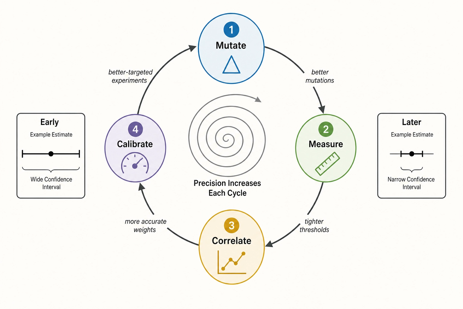
A property of this architecture that becomes visible only after the full chain is specified: the system produces compounding returns. Each experiment refines the calibration thresholds in Chapter 10. Better calibration improves the next experiment’s predictions - tighter JND thresholds mean the mutation engine can target smaller property changes with confidence that the change is perceptible, and better-calibrated confidence levels mean the correlation engine can weight its inputs more accurately. Better predictions enable better-designed experiments - the mutation engine can prioritize operators and magnitudes that earlier rounds showed to be most informative. Each round of mutate-measure-correlate-calibrate makes the next round’s inferences more precise. Early experiments operate with wide confidence intervals and v1 placeholder thresholds; later experiments operate with empirically grounded thresholds and accumulated causal-graph context. The framework is designed to get better with use, and the rate of improvement is itself an empirical quantity the calibration governance framework tracks.
Bibliography
[1] Berlyne, D. E. Conflict, Arousal, and Curiosity. McGraw-Hill, 1960. [BOOK] Used in: section 4 (inverted-U hypothesis relating stimulus complexity to positive response).
[2] Glasser, M. F., Coalson, T. S., Robinson, E. C., Hacker, C. D., Harwell, J., Yacoub, E., … & Van Essen, D. C. A Multi-Modal Parcellation of Human Cerebral Cortex. Nature, 536(7615), 171-178, 2016. [EMPIRICAL] Used in: sections 1-4 (360-area cortical parcellation used by Vₙ throughout this chapter).
[3] Kay, K. N., Naselaris, T., Prenger, R. J., & Gallant, J. L. Identifying Natural Images from Human Brain Activity. Nature, 452(7185), 352-355, 2008. [EMPIRICAL] Used in: section 1 (foundational encoding-model work underlying the Vₙ prediction pipeline).
[4] Nishimoto, S., Vu, A. T., Naselaris, T., Benjamini, Y., Yu, B., & Gallant, J. L. Reconstructing Visual Experiences from Brain Activity Evoked by Natural Movies. Current Biology, 21(19), 1641-1646, 2011. [EMPIRICAL] Used in: section 1 (extension of encoding models to natural video stimuli, methodological basis for TRIBE v2).
[5] Yue, X., Vessel, E. A., & Biederman, I. Lower-Level Stimulus Features Strongly Influence Responses in the Fusiform Face Area. Cerebral Cortex, 21(1), 35-47, 2011. [JOURNAL] Used in: section 1, section 2 (FFA response modulation by stimulus features such as face size, grounding the face-area-to-FFA-activation link).
[6] Bretherton, B., Deuchars, J., & Windsor, W. L. The Effects of Controlled Tempo Manipulations on Cardiovascular Autonomic Function. Music & Science, 2, 1-16, 2019. [JOURNAL] Used in: section 5 (tempo changes drive involuntary cardiovascular responses, supporting bypass-mediated arousal pathway).
[7] Chee, T., et al. The Effects of Music and Auditory Stimulation on Autonomic Arousal, Cognition and Attention: A Systematic Review. International Journal of Psychophysiology, 199, 112328, 2024. [SYSTEMATIC REVIEW] Used in: section 5 (systematic evidence that auditory stimulation modulates autonomic arousal without conscious mediation).
[8] Corbetta, M., & Shulman, G. L. Control of Goal-Directed and Stimulus-Driven Attention in the Brain. Nature Reviews Neuroscience, 3(3), 201-215, 2002. [REVIEW] Used in: section 4 (established role of the dorsal attention network in voluntary attention allocation).
[9] Heimann, K. S., et al. “Cuts in Action”: A High-Density EEG Study Investigating the Neural Correlates of Different Editing Techniques in Film. Cognitive Science, 41(6), 1555-1588, 2017. [JOURNAL] Used in: section 4 (EEG evidence of frontal attention-network engagement during film cuts).
[10] Cutting, J. E., DeLong, J. E., & Nothelfer, C. E. Attention and the Evolution of Hollywood Film. Psychological Science, 21(3), 432-439, 2010. [JOURNAL] Used in: section 4 (attention allocation tracks editing rate evolution in Hollywood film).
[11] Gold, B. P., et al. Predictability and Uncertainty in the Pleasure of Music: A Reward for Learning? Journal of Neuroscience, 39(47), 9397-9409, 2019. [JOURNAL] Used in: section 4 (quadratic inverted-U effects of information content on liking, supporting Berlyne’s framework in a related perceptual domain).